Integrazione Numerica di Equazioni Differenziali: 50 anni fa l’uomo ha messo piede sulla Luna. Parte II

Questo è il secondo articolo di questa serie dedicata alla soluzione numerica delle equazioni differenziali. La serie prende spunto dagli eventi che hanno portato l’uomo sulla Luna.

Nel luglio del 2019, quando ho iniziato a scrivere questo articolo, ricorreva il 50esimo anniversario della missione Apollo 11 (Neil A. Armstrong, Edwin A. Aldrin and Michael Collins) in cui gli astronauti Armstrong, Aldrin hanno posato il piede sulla superficie lunare. Un evento epocale nella storia umana che segna anche l’inizio della esplorazione spaziale. Dopo 50 anni, la NASA come altre agenzia spaziali e compagnie private, si stanno preparando per tornare sulla Luna per creare avamposti per l’esplorazione umana di pianeti più distanti come per esempio Marte. Questo anniversario mi portò ad interessarmi per raccogleire idee per la mia attività d’insegnamento e per curiosità personale, alle tecniche d’integrazione numerica delle equazioni differenziali usate per effettuare i calcoli delle traiettorie dal sistema di guida delle astronavi Apollo e dai calcolatori che hanno assistito l’impresa dalla Terra. In questo articolo semi divulgativo riassumo le informazione che ho raccolto leggendo (in maniera incompleta) la documentazione della NASA e quella ottenuta leggendo dei libri sull’argomento. Come mio solito presenterò anche dei semplici programmi che implementano questo algoritmi.

Continue reading →

Molecular Machines: the Coronavirus SARS-CoV-2 Menace. Part I

“If you know the enemy and know yourself, you need not fear the result of a hundred battles. If you know yourself but not the enemy, for every victory gained you will also suffer a defeat. If you know neither the enemy nor yourself, you will succumb in every battle.”

SunTzu. The Art of War

A virus is the Bauhaus of the form of life: the minimalist reduction of an organism to its essential element of functionality. More pragmatically, it is a container of genetic code provided with a smart mechanism that allows it to invade cells of another host organism. As a molecular machine, a virus can resemble in shape and destructive power the Death Star spaceship of the Star War saga. Therefore, it is a molecular machine that we do not definitively want to have within us!

The spread of the coronavirus SARS-CoV-2 has produced a new pandemic, i.e. an infection caused by a pathogen that affects the entire population of a living species, in this case the human one. This global emergency situation is the result of a natural competition between living species that reminds us that we are still a small brick of the Gaia ecosystem. However, although it is always difficult to believe given the state in which we have reduced our planet, we are the most intelligent life form in the known universe. So it would be quite embarrassing to be defeated by an invisible enemy.

Continue reading →

Examples of the Particle in a Box Model Applications

In a previous article, I have shown a simple derivation of the properties of a quantum particle confined in a one-dimensional box. Although the model is straightforward with unrealistic assumptions, such as the infinite walls, it produced qualitative results that paved the way for the development of quantum chemistry. There are several example practical applications in chemistry and nanoscience where the particle in a box model can be applied or serves as a conceptual foundation.

Continue reading →

Physical Chemistry. The Particle in a Box I: the Schrödinger Equation in One-dimension

In 1926, the Austrian physicist Erwin Schrödinger (1887-1961) made a fundamental mathematical discovery that had a profound impact on the study of the molecular world (in 1933, Schrödinger was awarded the Nobel Prize in Physics just seven years later, his breakthrough discovery). He discovered that a quantum system’s state composed of particles (such as electrons and nucleons) could be described by postulating the existence of a function of the particle coordinates and time, called state function or wave function (\Psi, psi function). This function is the solution of a wave equation: the Schrödinger equation (SE). Although the SE equation can be solved analytically only for relatively simple cases, the development of computer and numerical methods has made possible the application of SE to study complex molecules. 

Continue reading →

A personal tribute to one of the founders of MD simulation of biological molecules: Prof Herman J.C. Berendsen (1934-2019)

Subscribe to continue reading

Subscribe to get access to the rest of this post and other subscriber-only content.

The First 150 Years of the Periodic Table of the Elements

That the nobility of man, acquired in a hundred centuries of trial and error, lay in making himself the conquerer of matter, and that I had enrolled in chemistry because I wanted to remain faithful to this nobility. That conquering matter is to understand it, and understanding matter is necessary to understanding the universe and ourselves: and that therefore Mendeleev’s Periodic Table, which just during those weeks we were laboriously learning to unravel, was poetry, loftier and more solemn than all the poetry we had swallowed down in liceo; and come to think of it, it even rhymed!

Primo Levi, The Periodic Table.

This year marks the 150th anniversary of the periodic table of the elements (TPE) which currently has 118 entries, the latest arrival (the Tennessine) was discovered 10 years ago (announced in April 2010), and I feel obliged as a chemist to give some a small informative contribution to celebrate this important event.

Continue reading →

L’Integrazione Numerica di Equazioni Differenziali: 50 anni fa l’ uomo ha messo piede sulla Luna

Nel giorno in cui iniziai a scrivere questo articolo ricorreva l’anniversario della prima esplorazione da parte dei cosmonauti americani Neil Armstrong, Michael Collins, Buzz Aldrin della nostra Luna. Anche se non ho una memoria diretta di questi eventi, le missioni delle progetto Apollo evocano in tutti noi una forte emozione rappresentando un momento unico ed epico nella storia della conquista dello spazio. Nessun altro uomo ha messo di nuovo piede sulla Luna dopo l’ultima missione (Apollo 17) nel 1972, per cui i recenti annunci della NASA di nuove esplorazioni umane del nostro satellite rende l’anniversario ancora più eccitante.

L’ immagine di copertina di questo articolo è stata creata da mio figlio Leonardo per una sua ricerca scolastica sulle missioni Apollo ed è un collage d’immagini ottenute usando i programmi Google Earth e Sketchup. Nella figura si confrontano le dimensioni del razzo Saturno V con quelle della meravigliosa cattedrale di Lincoln in Gran Bretagna per dare un’idea dell’enorme grandezza del vettore spaziale. Il pensiero che l’uomo sia riuscito nel giro pochissimi anni in uno sforzo tecnologico e scientifico immenso a costruire questa cattedrale volante della tecnologia mi ha suscitato una forte curiosità a cui non ho saputo trattenermi e ho così iniziato a spiluccare la miriade di documenti disponibili sul sito della NASA sul programma Apollo nella ricerca di qualche aspetto interessante e curioso di questa impresa tecnologica senza eguali.

Continue reading →

The Logistic Map and the Feigenbaum Constants: a Retro Programming Inspired Excursion

“… Mitchell Feigenbaum was an unusual case. He had exactly one published article to his name, and he was working on nothing that seemed to have any particular promise. His hair was a ragged mane, sweeping back from his wide brow in the style of busts of German composers… At the age of twenty he had already become a savant among savants, an ad hoc consultant [at Los Alamos National Laboratory, USA] whom scientist would go to see about any expecially intractable problem.”

James Gleick, Chaos: the amazing science of the unpredectable.

This year, on June 30th 2019, Mitchell J. Feigenbaum died at the age of 74. Feigenbaum was an American mathematician that became famous with the discovery of the universal constants that bear his name. In the middle of the ’80, reading Le Scienze magazine (the Italian edition of Scientific American) I got to know of the contribution to the chaos theory of this charismatic mathematician. In particular, I was delighted by reading the Douglas Hofstadter’s article in the rubric “Temi Metamagici” ( Methamagical themes) (Scientific American, November 1981). The article explained the emergence of the chaos in the iteration map of the logistic equation, the same equation deeply studied by Feigenbaum. The full story about the Mitchell Feigenbaum and his discovery of his universal constants is delightly narrated in the beautiful book Chaos:the amazing science of the unpredectable by J. Gleick [1]. Here it is just another small extract:

“… in the summer of 1975, at a gathering in Aspen, Colorado, he heard Steve Smale [another key mathematicial in the developing of the chaos theory, NDA] talk about some of the mathematical qualities of the same quadratic difference equation [the same studied by Robert May, NDA]. Smale seemed to think that there were some interesting open questions about the exact point at which the mapping changes from periodic to chaotic. As always, Smale had a sharp instinct for questions worth exploring. Feigenbaum decided to look into it once more.”[1]

Continue reading →

Numerical Integration of Differential Equations. Part I.: Katherine Johnson and the Euler’s Method.

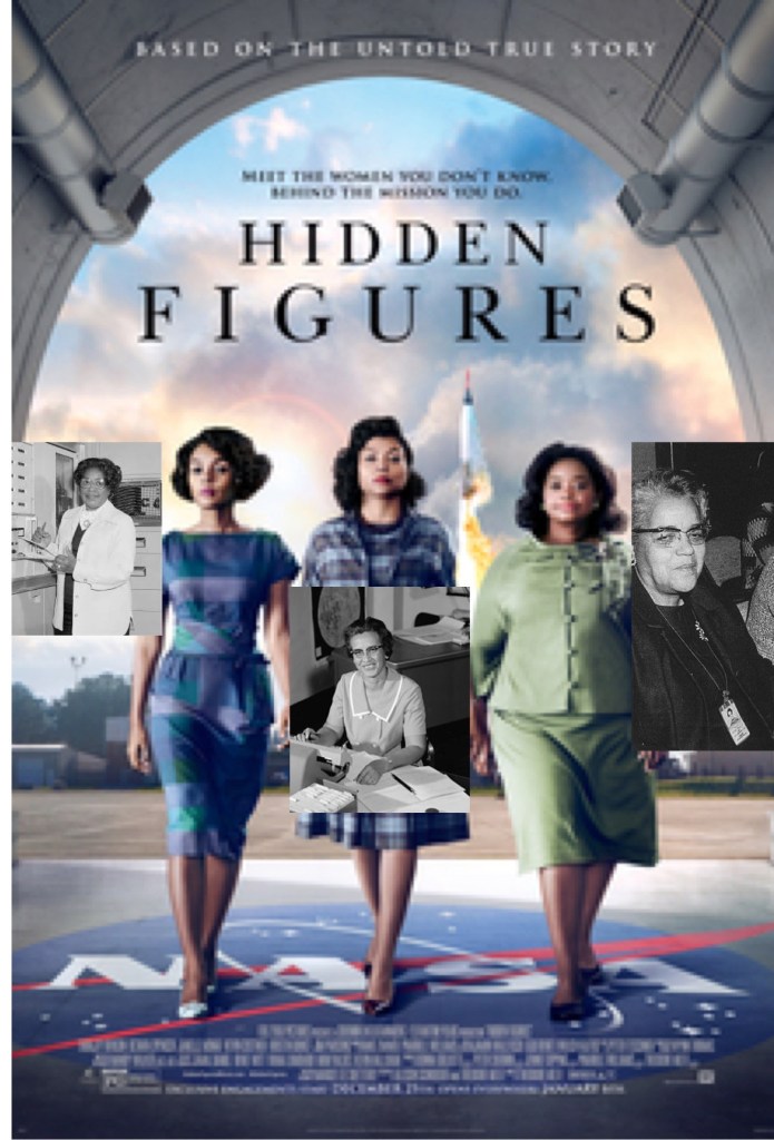
This article was inspired by the beautiful 2016 movie Hidden Figures (based on the book of the same name by M. L. Shetterley) which tell the dramatic story of three talented black women scientist that worked as “human computers” for NASA in 1961 for the Mercury project.

Figure 1: Official theatrical poster of the movie and the phFoto of the real protagonist. From left to right. Mary Jackson, Katherine Goble and Dorothy Vaughan. (source: wikipedia)

In the movie, the mathematician Creola Katherine Johnson (or Globe) (interpreted by Taraji P. Henson), had a brilliant intuition on how to numerically solve the complex problem to find the transfer trajectory for the reentry into the Earth atmosphere of the Friendship 7 capsule with the astronaut John Glenn on board. In the particular scene, she was standing together with other engineers and the director of the Langley Research Center (a fictional character interpreted by Kevin Coster) in front of the vast blackboard looking to graph and equations when she says that the solution might be in the “old math” and she runs to take an old book from a bookshelf with the description of the Euler method [UPDATE, May 2022: I just come across another excellent youtube video by the Tibees about the mathematical work of K. Johnson at NASA, and at the end of the video she reveal that the book shown in the movie is the classic H Margenau & G. M Murphy, The Mathematics of Physics and Chemistry. Published by Van Nostrand, 1956]. The scene is also nicely described in the youtube video lesson by Prof. Alan Garfinkel of the UCLA. A detailed description of the numerical solution based on the original derivation of K. Johnson is in the Wolfram blog website.

Katherine Globe was using for these complex calculation her brilliant brain with the support of a mechanical calculator (the Friden STW-10, in the movie, this machine is visible in different scenes). In a scene of the film, she revealed that her typical computing performance was of 10000 calculations per day and probably for calculations, she was not referring to single arithmetic operations! These exceptional mathematical skills have given a significative contribution at the beginning of the American space program, but it became insufficient to handle the more complex mathematics necessary to land the man on the Moon, and the other fantastic NASA achievements.

Continue reading →

The Calculation of the Lattice Energy: The Born-Haber Cycle

My blog in italian on this topics is very popular and for this reason I decided to add an English translation (when I have some free time, I will also translate the text in the Figure and Table). So be tune and more will come!

The stability of a crystal lattice at constant T and P conditions is linked to the Gibbs free energy of lattice formation by the relations

M^+ (g) + X^- (g) \rightarrow MX (s) \hfill  (1)

\displaystyle \Delta G^{\circ} = \Delta H^{\circ} - T \Delta S^{\circ} \hfill  (2)

If {\Delta G^{\circ}} is more negative for the formation of the {I} structure than for the {II} structure, the {II \rightarrow I} transition will be spontaneous and the solid will have that structure.

Continue reading →