Houston, Tranquillity Base here. The Eagle has landed.

Neil Armstrong, 20 July 1969

This article is also dedicated to the memory of Margaret Hamilton (1936–2026), whose pioneering work in software engineering contributed to the success of the Apollo missions.

This is the second article in a series introducing numerical methods for solving differential equations, inspired by one of humanity’s greatest technological achievements: the journey to the Moon.

In July 2019, I wrote the Italian version of this article to celebrate the 50th anniversary of the Apollo 11 mission. On 20 July 1969, Neil Armstrong and Edwin “Buzz” Aldrin became the first humans to walk on the lunar surface, while Michael Collins remained in lunar orbit aboard the Command Module Columbia.

More than half a century later, the Moon continues to inspire scientists, engineers, and explorers. NASA’s Artemis programme, together with initiatives from other space agencies and private companies, represents a renewed effort to explore our nearest celestial neighbour. In 2026, the Artemis II mission marked another milestone with a crewed journey around the Moon, recalling the historic flight of Apollo 8 in 1968. These developments renewed my interest in the mathematical and computational techniques that made the Apollo missions possible. How could the computers of the 1960s, with their extremely limited memory and processing power, calculate the trajectories necessary to navigate between the Earth and the Moon?

To explore this question, I returned to historical NASA documentation and the scientific literature on numerical integration. In this article, I summarise some of these findings and introduce the Runge–Kutta method, one of the most widely used techniques for solving differential equations numerically. As usual, I will also include a simple computer program to illustrate how these mathematical ideas can be put into practice.

Numerical integration in the guidance system of the spacecraft during the Apollo missions

Before launching the Apollo 11 mission to the Moon, NASA scientists had to refine the precise position of the Moon in its orbit using radar and satellite measurements. This information was crucial to enable the onboard computer of the Apollo modules to navigate towards the Moon with high accuracy, execute the correct insertion into the trans-lunar orbit, land, and complete subsequent phases of the return to Earth orbit. Moreover, the early Apollo missions 8 and 10 provided data for further adjustments that accounted for lunar gravitational anomalies for both the circumlunar orbit insertion and the descent of the lunar module (LEM). All Apollo missions were equipped with two compact and powerful computers at the time (known as Apollo Guidance Computers or AGC), one in the command module and one in the LEM.

These technological marvels were conceived at the prestigious MIT (Massachusetts Institute of Technology). To reduce space, the first integrated circuits were utilized (the NASA commission provided a significant initial boost to the development and commercialization of this technology) and magnetic core memories that ensured maximum reliability under mission conditions. It is astounding to think that these engineering gems, which cost millions of dollars, had computing power and memory only slightly exceeding one of the first home computers (for example, the Commodore 64), built in the decade following the last Apollo missions and marketed at a cost one million times lower! Like the home computers of the 1980s, the AGC was equipped with a processor with a clock frequency of about 2 MHz. The read-only memory (ROM) containing the “operating system” of the AGC was called “Core Rope Memory” or “LOL memory” (Little Old Lady memory). This type of memory was a read-only memory system based on intertwined ropes with magnetized wires, and each program was manually coded by a group of women, contributing to the name “Little Old Lady” for the memory. The total capacity of the AGC’s ROM was about 36,864 words of 15 bits each. Using the aforementioned conversion (1.875 bytes per word), it can be calculated that the AGC’s ROM was approximately 69.12 kilobytes (36,864 words x 1.875 bytes/word). The AGC used a volatile memory known as “Random Access Memory” (RAM). The AGC’s RAM was divided into two main types:

The Apollo Guidance Computer used two principal types of memory:

1. Fixed Memory (ROM): Approximately 36,864 words of 16 bits each, including the parity bit, corresponding to about 72 KB. This non-volatile memory stored the flight programs and was implemented using the remarkable core rope memory technology.
2. Erasable Memory (RAM): Approximately 2,048 words of 16 bits each, including the parity bit, corresponding to about 4 KB. This magnetic-core memory was used to store temporary data and variables during program execution.

Astonishingly, such sophisticated navigation and guidance operations could be performed with only about 4 KB of working memory! An interesting article by B. Hayes on the AGC can be found in reference [1].

Margaret Hamilton: The woman behind the Apollo software

The software that controlled these computers was another remarkable achievement of the Apollo programme. One of the key figures behind its development was Margaret Hamilton (1936–2026), the pioneering computer scientist who led the team responsible for the onboard flight software at MIT. Hamilton, who passed away in September 2026, was among the first to recognise that software development required the same engineering discipline and reliability standards as the hardware itself. Her contributions helped establish the foundations of modern software engineering.

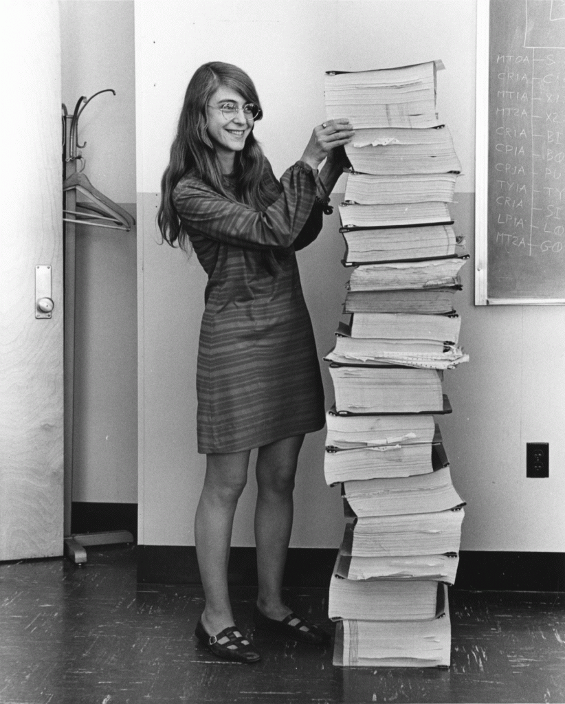
The ingenuity of Hamilton and her team was dramatically demonstrated during the first Moon landing in July 1969. As the Lunar Module Eagle descended towards the lunar surface, the Apollo Guidance Computer unexpectedly displayed the now-famous alarm codes 1201 and 1202. The problem was associated with additional processing demands from the rendezvous radar system, which overloaded the computer’s available processing capacity. Fortunately, the software had been designed to prioritise essential tasks and recover from such situations without losing the critical guidance functions. Thanks to this fault-tolerant design, Mission Control was able to authorise Armstrong and Aldrin to continue their descent. The Eagle landed safely on the Moon on 20 July 1969. It is fascinating to compare this achievement with modern computers. I once timed the reboot of my 2012 MacBook Pro, equipped with a solid-state drive: it took approximately 44 seconds! Of course, the AGC’s rapid recovery was fundamentally different from restarting a modern operating system, but the comparison gives an impression of the extraordinary demands placed on the Apollo software. Imagine waiting 44 seconds for a computer to restart while descending towards the lunar surface!

Hamilton’s contribution was recognised in 2016 when she received the Presidential Medal of Freedom. Her recent passing offers an opportunity to remember that the success of the Apollo missions depended not only on the astronauts and spacecraft engineers, but also on the mathematicians and programmers whose work made the journey possible.

The software that controlled them was a gem of ingenuity. Capable of multitasking, it could monitor various sensors and servomechanisms in real-time. History shows that the robustness of this control program was tested during the first moon landing in July 1969. Due to a (human) error, the radar for detecting the position of the Command Service Module (CSM) was left on during the descent. During the landing, although it wasn’t detecting the CSM, the radar continued to flood the AGC’s memory with data. In response, the AGC alerted Armstrong and Collins with the famous alarm code 1202, indicating a memory overload caused by the high frequency of telemetry readings. However, not knowing exactly what the problem was, NASA gave the go-ahead to continue the mission since the operating system could overcome stall conditions due to overload simply by rebooting the computer! We know well that rebooting a Windows/MacOS/Linux system takes much longer than a fraction of a second! I timed the reboot of my MacBook Pro (2012 version) whose OS is installed on a solid-state drive (the AGC also uses solid-state memory but is times less capacious: 44 seconds. I leave it to you to consider the consequences of such a slow reboot, given that the alarm code 1202 appeared several times when the landing module was about 2 km from the surface.

From Apollo Guidance to Numerical Integration

Despite its remarkable capabilities, the AGC remained severely constrained by its limited memory and processing power. Consequently, the selection of efficient and accurate numerical algorithms was essential for the navigation and guidance operations required during the Apollo missions.

Among the most computationally demanding operations were the navigation calculations performed during coasting, when the spacecraft travelled without continuous propulsion. Particularly important was the calculation of trajectories between the Earth and Moon, including the return journey. These calculations required the guidance computer to predict the spacecraft’s motion under the gravitational influence of several celestial bodies.

One interesting aspect of the Apollo navigation system was the representation of the positions of the Moon and Sun using polynomial approximations. Rather than repeatedly calculating their orbital motion from first principles, the computer could evaluate previously determined coefficients stored in its fixed memory.

For example, the position of the Moon relative to the Earth could be approximated by a ninth-degree polynomial for each Cartesian coordinate:

Here, , , and represent the coordinates of the Moon at time , measured relative to a reference epoch near the middle of the mission. The polynomial coefficients were determined before launch and provided an efficient approximation over a limited time interval [2].

Knowing the positions of the celestial bodies was only part of the problem. The computer also had to predict how their gravitational attraction would influence the spacecraft’s trajectory.

This required solving the equations of motion using numerical integration.

The Apollo navigation software employed specialised algorithms adapted to orbital mechanics, including methods related to the Runge–Kutta family and the work of the mathematician Evert Johannes Nyström [3,4]. The precise historical implementation differed from the classical fourth-order Runge–Kutta method described below, but the underlying principle of advancing a numerical solution through successive time steps provides a useful introduction.

The Runge–Kutta method

In the previous article, we introduced Euler’s method, one of the simplest techniques for solving ordinary differential equations (ODEs). Although easy to implement, Euler’s method can accumulate substantial numerical errors, particularly when relatively large integration steps are used.

The Runge–Kutta family of methods provides a more accurate alternative. Instead of estimating the solution using only the slope at the beginning of each time interval, these methods evaluate the behaviour of the function at several intermediate points.

One of the most widely used examples is the classical fourth-order Runge–Kutta method, commonly abbreviated as RK4.

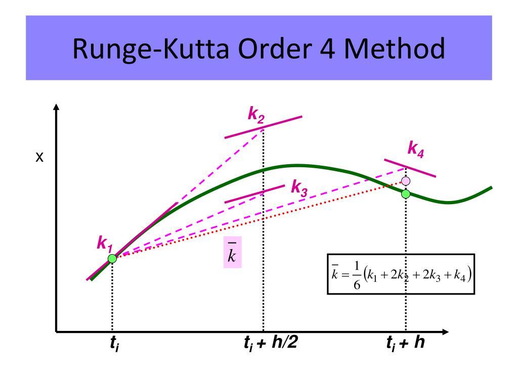
Consider a first-order differential equation:

where is the unknown function and describes its rate of change.

The RK4 algorithm evaluates four intermediate quantities:

Here, is the integration time step, is the current time, and is the approximate solution at that time.

The four contributions are combined to calculate the next value:

The procedure is repeated to advance the numerical solution through time.

The advantage of RK4 is that it generally provides considerably better accuracy than Euler’s method for the same step size. However, this improvement comes at a computational cost: four evaluations of the function are required for each step instead of one. This trade-off between computational efficiency and numerical accuracy was particularly important when computers had only a few kilobytes of memory and limited processing power.

Extending RK4 to planetary motion

The same numerical procedure can be extended to systems containing several coupled differential equations.

For example, the motion of a body in three-dimensional space is described by its position and velocity, which change under the influence of gravitational forces.

Instead of treating each variable separately, we can combine them into a single vector:

The equations of motion can then be expressed compactly as:

The RK4 algorithm applies to this vector in exactly the same way as to a single differential equation. Each of the four intermediate quantities becomes a vector, and the solution is advanced using:

This compact formulation avoids writing separate equations for every coordinate and velocity component.

By specifying the gravitational forces acting on the bodies, the method can be used to simulate planetary orbits, satellite trajectories, and other dynamical systems.

In the next section, we will see how this approach can be implemented in a simple QB64 BASIC program to simulate the motion of planets in the Solar System.

IMPLEMENTATION IN THE PLANETARY PROGRAM

The following code snippet in QB64 BASIC calculates approximate solutions using the RK4 method and can be inserted into the PLANETARY program for simulating the orbits of the planets in the solar system presented in a previous article (in English).

For K = 1 To N
    MASS(K) = MASS(K) * MU
    X(K) = X1(K) * AU
    Y(K) = Y1(K) * AU
    Z(K) = Z1(K) * AU
    VX(K) = VX1(K) * VCV
    VY(K) = VY1(K) * VCV
    VZ(K) = VZ1(K) * VCV
Next K

' Inizia la simulazione
For T = 1 To NSTEPS
    For I = 1 To N
        ' Runge-Kutta Step 1
        KX1 = VX(I) * DT
        KY1 = VY(I) * DT
        KZ1 = VZ(I) * DT
        KVX1 = AX(I) * DT
        KVY1 = AY(I) * DT
        KVZ1 = AZ(I) * DT

        ' Runge-Kutta Step 2
        X2 = X(I) + 0.5 * KX1
        Y2 = Y(I) + 0.5 * KY1
        Z2 = Z(I) + 0.5 * KZ1
        VX2 = VX(I) + 0.5 * KVX1
        VY2 = VY(I) + 0.5 * KVY1
        VZ2 = VZ(I) + 0.5 * KVZ1
        AX2 = 0
        AY2 = 0
        AZ2 = 0
        For J = 1 To N
            If (J <> I) Then
                D2 = (X2 - X(J)) ^ 2 + (Y2 - Y(J)) ^ 2 + (Z2 - Z(J)) ^ 2
                ID = 1 / Sqr(D2)
                F = G * MASS(J) / D2
                AX2 = AX2 + F * (X(J) - X2) * ID
                AY2 = AY2 + F * (Y(J) - Y2) * ID
                AZ2 = AZ2 + F * (Z(J) - Z2) * ID
            End If
        Next J
        KVX2 = AX2 * DT
        KVY2 = AY2 * DT
        KVZ2 = AZ2 * DT

        ' Runge-Kutta Step 3
        X3 = X(I) + 0.5 * KX2
        Y3 = Y(I) + 0.5 * KY2
        Z3 = Z(I) + 0.5 * KZ2
        VX3 = VX(I) + 0.5 * KVX2
        VY3 = VY(I) + 0.5 * KVY2
        VZ3 = VZ(I) + 0.5 * KVZ2
        AX3 = 0
        AY3 = 0
        AZ3 = 0
        For J = 1 To N
            If (J <> I) Then
                D2 = (X3 - X(J)) ^ 2 + (Y3 - Y(J)) ^ 2 + (Z3 - Z(J)) ^ 2
                ID = 1 / Sqr(D2)
                F = G * MASS(J) / D2
                AX3 = AX3 + F * (X(J) - X3) * ID
                AY3 = AY3 + F * (Y(J) - Y3) * ID
                AZ3 = AZ3 + F * (Z(J) - Z3) * ID
            End If
        Next J
        KVX3 = AX3 * DT
        KVY3 = AY3 * DT
        KVZ3 = AZ3 * DT

        ' Runge-Kutta Step 4
        X4 = X(I) + KX3
        Y4 = Y(I) + KY3
        Z4 = Z(I) + KZ3
        VX4 = VX(I) + KVX3
        VY4 = VY(I) + KVY3
        VZ4 = VZ(I) + KVZ3
        AX4 = 0
        AY4 = 0
        AZ4 = 0
        For J = 1 To N
            If (J <> I) Then
                D2 = (X4 - X(J)) ^ 2 + (Y4 - Y(J)) ^ 2 + (Z4 - Z(J)) ^ 2
                ID = 1 / Sqr(D2)
                F = G * MASS(J) / D2
                AX4 = AX4 + F * (X(J) - X4) * ID
                AY4 = AY4 + F * (Y(J) - Y4) * ID
                AZ4 = AZ4 + F * (Z(J) - Z4) * ID
            End If
        Next J
        KVX4 = AX4 * DT
        KVY4 = AY4 * DT
        KVZ4 = AZ4 * DT

        ' Update positions and velocities using weighted average
        X(I) = X(I) + (1 / 6) * (KX1 + 2 * KX2 + 2 * KX3 + KX4)
        Y(I) = Y(I) + (1 / 6) * (KY1 + 2 * KY2 + 2 * KY3 + KY4)
        Z(I) = Z(I) + (1 / 6) * (KZ1 + 2 * KZ2 + 2 * KZ3 + KZ4)
        VX(I) = VX(I) + (1 / 6) * (KVX1 + 2 * KVX2 + 2 * KVX3 + KVX4)
        VY(I) = VY(I) + (1 / 6) * (KVY1 + 2 * KVY2 + 2 * KVY3 + KVY4)
        VZ(I) = VZ(I) + (1 / 6) * (KVZ1 + 2 * KVZ2 + 2 * KVZ3 + KVZ4)
        If (X(I) < LM And X(I) > -LM) And (Y(I) > -LM And Y(I) < LM) And (Z(I) < LZ And Z(I) > -LZ) Then
            PSet (225 + FX * X(I), 200 + FY * Y(I)), I
            PSet (575 + FX * X(I), 200 + FZ * Z(I)), I
        End If
    Next I

    R = R + DT
    DAYS = R * S2D
    Locate 32, 5: Print Using "TIME LAPSE: ######.## Days -> ####.## Years"; DAYS, DAYS * D2Y
    K$ = InKey$
    If K$ = "E" Or K$ = "e" Then SIGN = 1: RESCALE
    If K$ = "R" Or K$ = "r" Then SIGN = -1: RESCALE
Next T

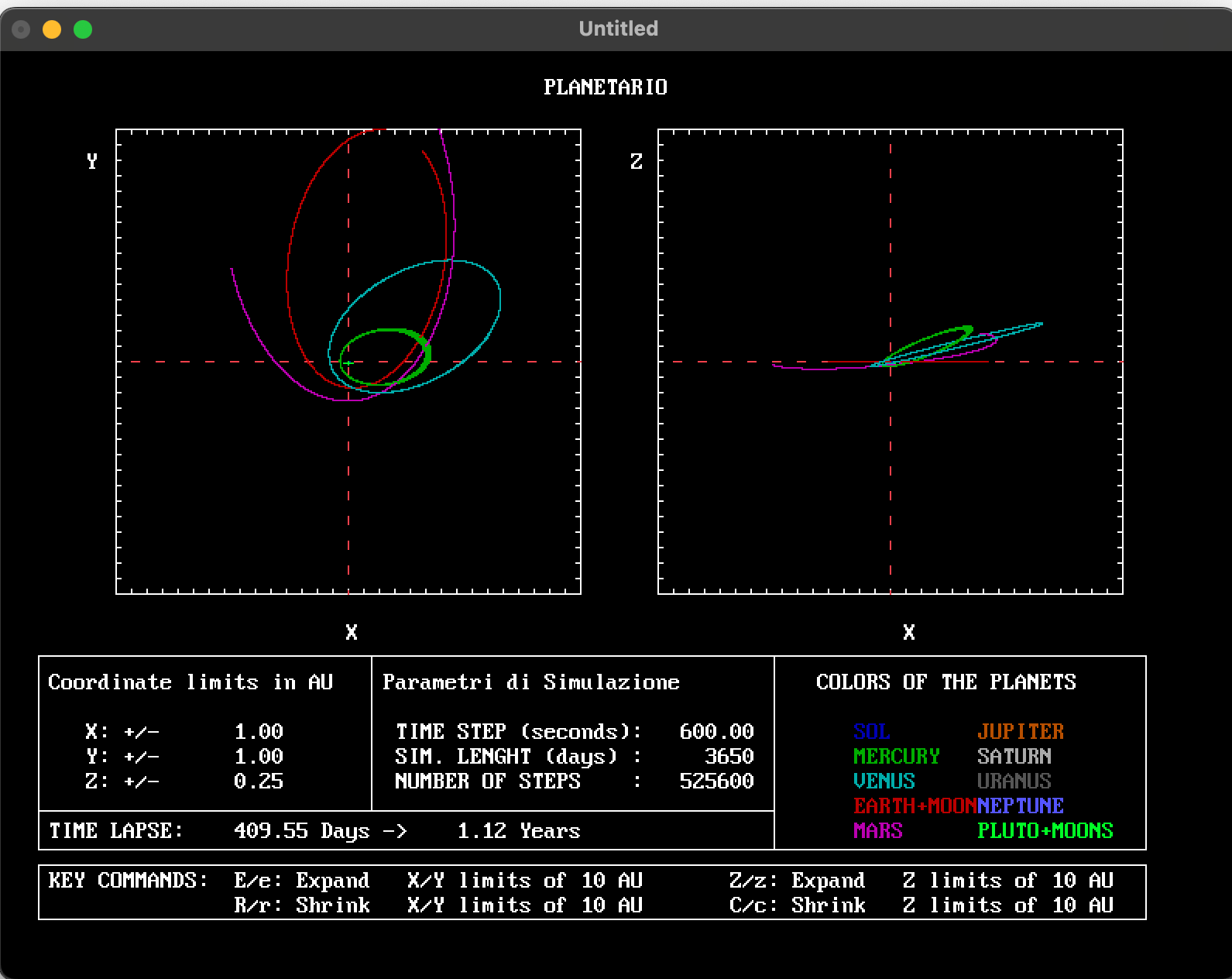
In the figure that follows, an example of simulation produced by the modified program is shown.

REFERENCES

1. Hayes, B. (2019). Moonshot Computing. American Scientist, May–June 2019. An engaging account of the Apollo Guidance Computer and its software.
2. Lunar Ephemeris Polynomials. Project Apollo – NASSP Documentation. A technical explanation of the polynomial approximations used to represent lunar positions.
3. Weinstock, M. (2016). Margaret Hamilton’s Apollo Code. MIT News, reproduced by NASA. Historical background on Hamilton and the Apollo flight software.
4. NASA (2003). Margaret Hamilton – NASA Honors Apollo Engineer. Recognition of Hamilton’s contributions to software engineering and fault-tolerant guidance systems.
5. NASA Apollo 11 Lunar Surface Journal. Apollo 11 Program Alarms. Historical discussion of the 1201 and 1202 alarms during the lunar landing.
6. MIT Instrumentation Laboratory. Guidance System Operations Plan for Luminary 1E, Section 5: Guidance Equations. Original technical documentation describing Apollo guidance equations, coasting integration, and Nyström numerical integration.