The Lissajous-Bowditch Curves |

Try to glue a small mirror to an end of a bent piece of wire fixed to a stable platform and let the laser beam of a laser pointer reflect on it. Entangled spires of an ephemeral dragon of light will perform a hypnotic dance on the wall of your room. This voluptuous dance is the results of two mutually perpendicular harmonic oscillations produced by the oscillations of the elastic wire.

The curved patterns are called Lissajous-Bowditch figures and named after the French physicist Jules Antoine Lissajous who did a detailed study of them (published in his Mémoire sur l’étude optique des mouvements vibratoires, 1857). The American mathematician Nathaniel Bowditch (1773 – 1838) conducted earlier and independent studies on the same curves and for this reason, the figures are also called Lissajous-Bowditch curves. Lissajous invented different mechanical devices consisting of two mirrors attached to two oriented diapasons (or other oscillators) by double reflecting a collimated ray of light on a screen, produce these figures upon oscillations of the diapasons. The diapason can be substituted with elastic wires, speakers, pendulum or electronic circuits. I the last case, the light is the electron beam of a cathodic tube (or its digital equivalent) of an oscilloscope. This blog is about these curves and shows demonstrations and applications.

Sinusoidal functions

The harmonic oscillations of the wire in the experiment described at the beginning of this blog can be mathematically described using sinusoidal functions defined in the time domain as

${f(t) = A \cos(\omega t - \phi)}$ .

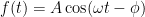
where the parameters ( ${A, \omega, \phi}$ ) have the following meanings:

${A}$ is the amplitude and it gives how high the graph ${f(t)}$ rises above the t-axis at its maximum values.
${\phi}$ is the phase lag and it indicates the position of the maximum of the function.
${\omega}$ is the angular frequency and it gives the number of complete oscillation of ${f(t)}$ in a time interval of length ${2\pi}$ .

The following useful quantities are associated with the previous parameters:

$\nu=\frac{\omega}{2 \pi}$ is the frequency of ${f(t)}$ and it represent the number of complete oscillation of ${f(t)}$ in a time interval of length 1.
${\tau=\phi/\omega}$ is the time delay or time shift and it indicates how far the graph of the ${\cos(\omega t)}$ has been shifted along the t-axis.
$\mathcal{P}=2\pi/\omega=1/\nu$ is the period and indicates the time required for one complete oscillation.

An example of sinusoidal functions is shown in Fig. 1.

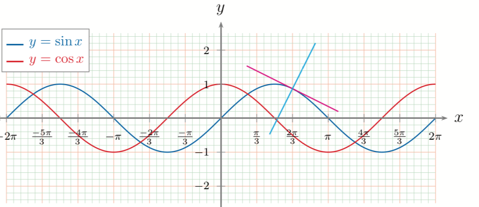
Fig. 1: Example of a trigonometric function.

In Fig. 2, two periodic functions having the same parameters but with a phase shift of $\Delta \phi=\pi/6$ are shown.

Screenshot 2018-11-09 at 19.52.12 — Fig. 2: The parameters for this function are ${A=7/4, \phi=\pi/6, \omega=3/2, \tau=\phi/\omega=\pi/9, \nu=\omega/2\pi=3\pi/4, P=1/\nu=4\pi.}$

Fig. 2: The parameters for this function are ${A=7/4, \phi=\pi/6, \omega=3/2, \tau=\phi/\omega=\pi/9, \nu=\omega/2\pi=3\pi/4, P=1/\nu=4\pi.}$

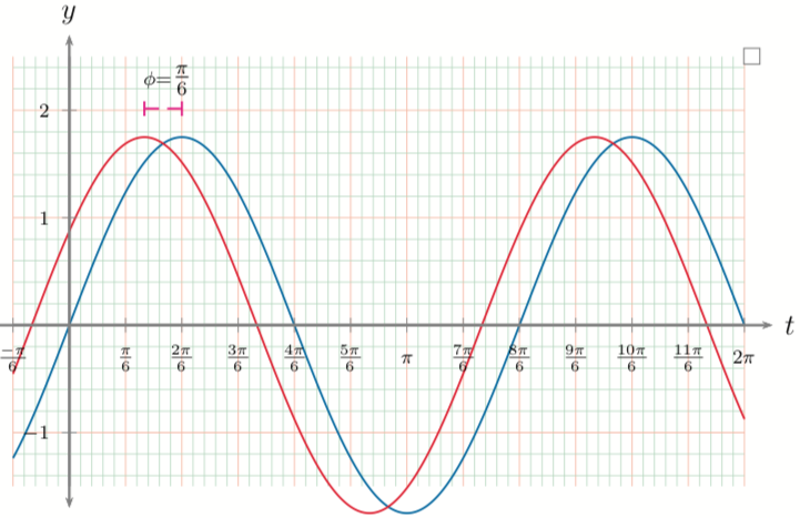
The Lissajous- Bowditch curves are generated by a parametric representation in the time variable $t$ of the two sinusoidal functions

$\begin{aligned} x &= A \sin (a t+ \delta) \\ y &= B \sin (b t) \end{aligned}$

By varying, the parameters $A, B, a, b$ and, ${\delta}$ , it is possible to obtain a variety of Lissajous-Bowditch curves with interesting properties. In Figure 3, some examples with $A = B = 1$ , and with $\delta = 0$ and ${\delta=50}$ in the first and second row, respectively, are shown.

Screenshot 2018-11-09 at 20.02.05 — Figure 3: Examples of Lissajous curves.

The kaleidophone

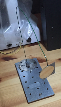
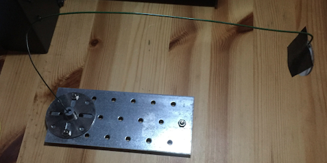
The simple experiment with the metallic wire described at the beginning of this blog was indeed a device invented by the physics Charles Wheatstone (1802-1875) – also well-known to electrical engineering for the Wheatstone’s bridge for the measure of the resistance – that called it a “Philosophical toy” but it is more properly named Kaleidophone [see references 1, 2, 3]. I have built one using some refuses materials: a squared metallic perforated plate as a base and a coated soft-iron wire for gardening bought in a hardware shop, a small circular mirror from a bricolage shop, and some other bits from a Meccano set (see the photos below). The wire can be also recycled from a dry cleaning coat hanger. You also need a laser pointer (I have used the one in a small laser level), a screen (for example a house door colored in white) and a good photo camera with the control of the shutter or a smartphone with the right apps! I have considered the last option using an iPhone 6 and the Slow Shutter apps.

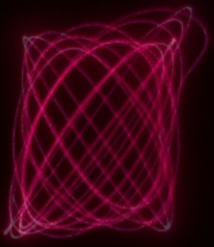
In the picture below, a preliminary example of Lissajous pattern produced by the Kaleidophone more to come…

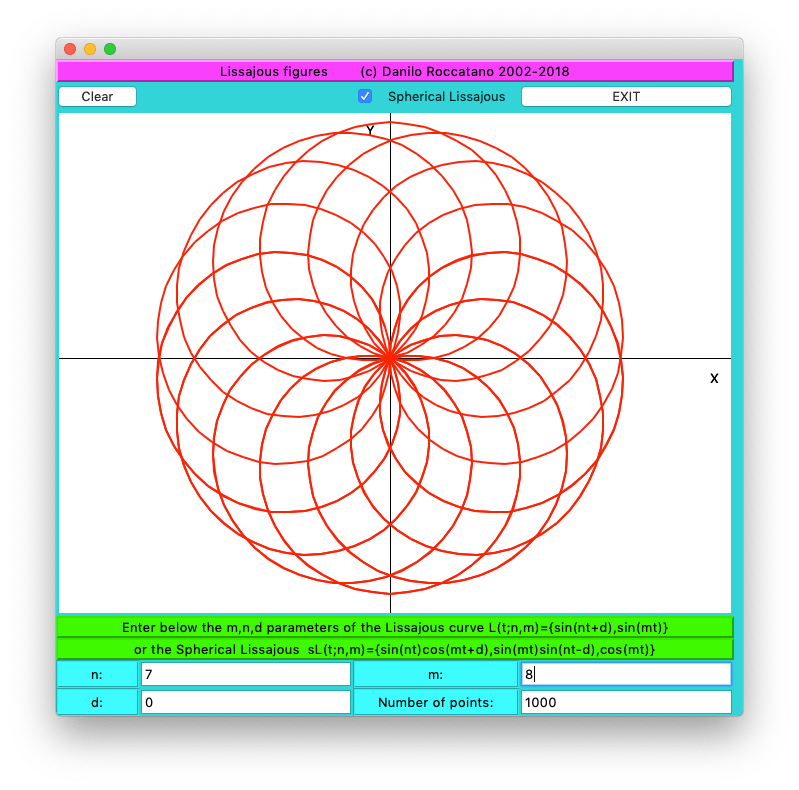
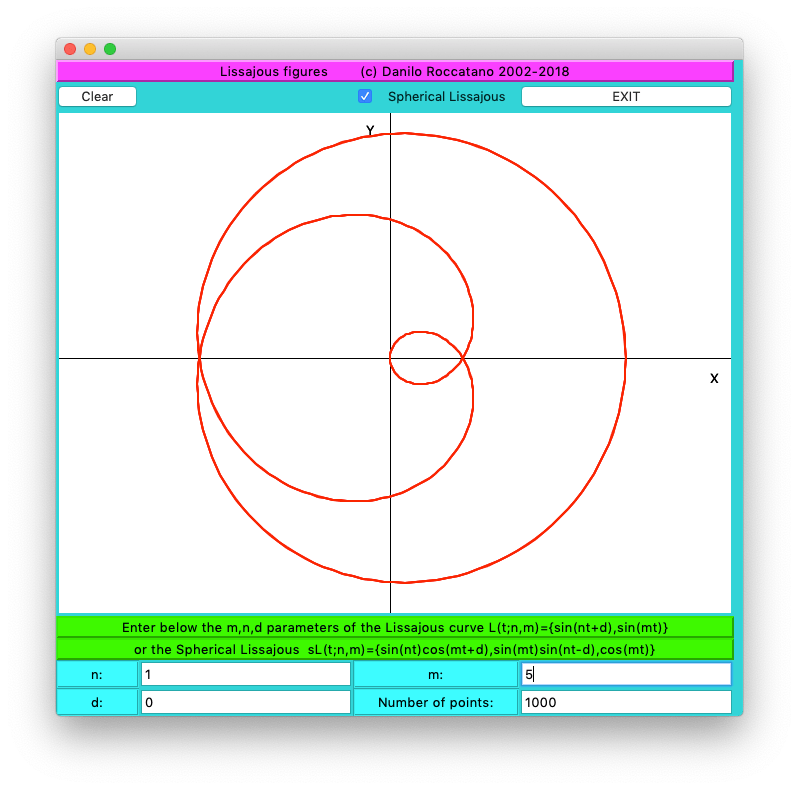
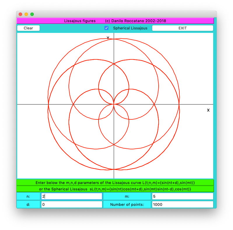
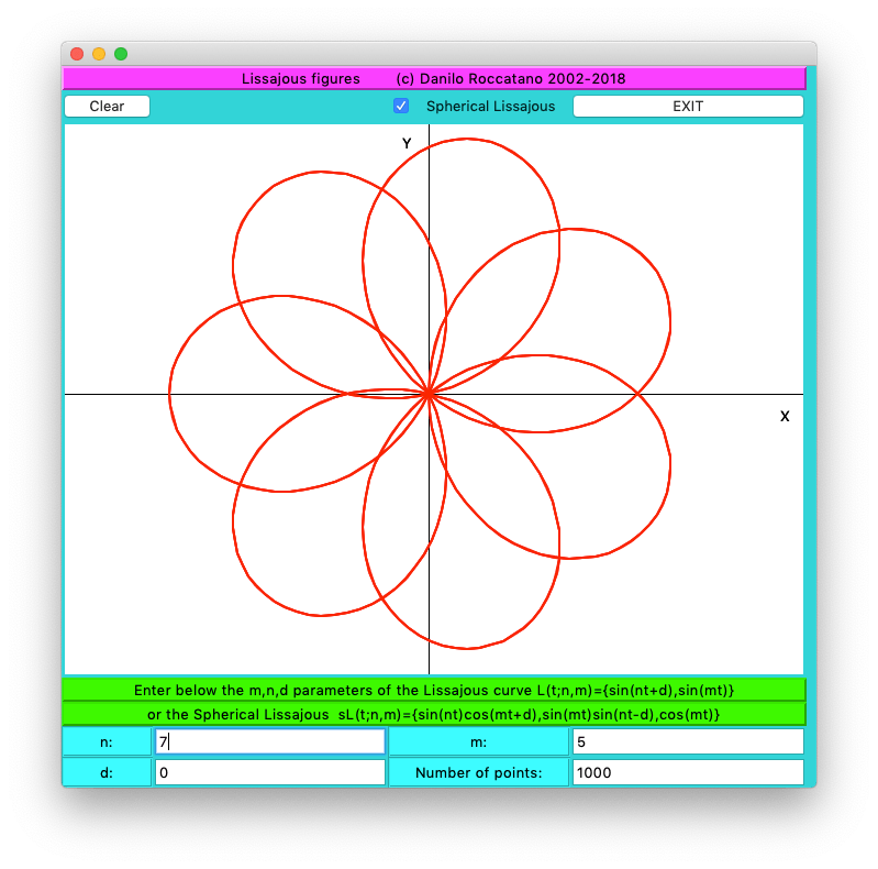
Spherical Lissajous curves

By reading the book “Computer and Imagination” by C. A. Pickover [4], I came across with an article that he wrote for the MIT press magazine Leonardo in the ’80 in which he gave a computational receipt for another beautiful occurrence of Lissajous figures, this time on the surface of a unit sphere. These figures are names spherical Lissajous curves and they are described as

$\boldsymbol{\ell}^{(\boldsymbol{m})}_{\alpha}(t) \equiv \begin{cases} x &= \sin(m_2 t) \cos (m_1 t - \alpha \pi), \\ y &= \sin(m_2 t) \sin (m_1 t - \textstyle\alpha \pi) \\ z &= \cos(m_2 t). \\ \end{cases} \quad t \in \mathbb{R}$

with $\boldsymbol{m} = (m_1, m_2) \in{\mathbb N}^{2}$ and a rotation parameter $\alpha \in {\mathbb R}.$

The curves $\boldsymbol{\ell}^{(\boldsymbol{m})}_{\alpha}$ are described on the unit sphere $S^2 = \{x,y,z \in \Re^3 : x^2+y^2+z^2 = 1\}$ . These tridimensional bi-parametric curves describe a superposition of a latitudinal and a longitudinal harmonic motion determined by the frequencies $(m_1,m_2)$ (see [5] for more information). There are several applications of these curves. Pickover, for example, have used them as a simple model to represent the morphology of complex seashell. In the same book, he also give a pseudocode to make computational experimentation with them projecting on the ${x,y}$ coordinates with the equations:

$L(t:m_1,m_2) = \{\sin(m_2 t) \cos(m_1 t), \sin(m_2 t) \sin(m_1 t)\}$

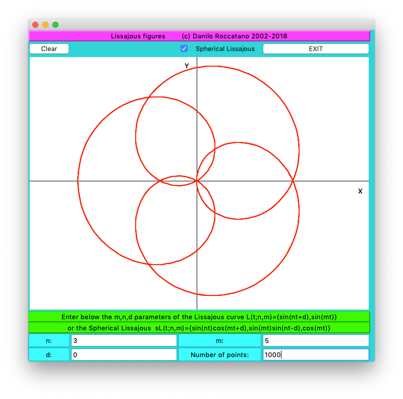
If the ratio $\frac{m_2}{m_1}$ is a rational number the resulting curve is closed otherwise, given infinity number of iteration, they will cover for all the points on the spherical surface.

I couldn’t resist myself but add these curves to the Tcl/Tk program reported in the appendix that I developed some time ago. Some example of output are reported below, note that the parameters are called $(n, m, d)$ instead of $(m_1, m_2, \alpha)$ .

Bibliography

R. J. Whitaker. The Wheatstone kaleidophone. American Journal of Physics 61, 722 (1993).
Thomas B. Greenslade Jr. All about Lissajous figures. The Physics Teacher 31, 364 (1993).
Thomas B. Greenslade Jr.Devices to Illustrate Lissajous Figures. The Physics Teacher 41, 351 (2003).
C.A. Pickover. Computer and Imagination. St. Martin’s Press; Reprint edition (1 Oct. 1992). The work of Pickover and its spherical Lissajous are also described by A.K. Dewdney in one of his article in Computer Recreations (Scientific American January 1991, also reprinted in his book “The TinkerToy Computer”).
https://www.math.unipd.it/~erb/LSphere.html.

Appendix

A program to generate Lissajous-Bowdich figures

The following Tcl/Tk program allow you to explore the Lissajous-Bowdich curves. The program was developed under MacOSX but it should work also under Linux.

# /bin/sh
# the next line restarts using wish \
exec wish "$0" "$@"
# 
#======================================================================
#  DESCRIPTION: 2D and 3D Lissajous-Bowdich curve generator 
#======================================================================               
#  DEVELOPED USING: tcl/tk 
#   
#======================================================================
# Author:        Danilo Roccatano 
# Version:       1.0
# Copyright (C): 2018-2020 Danilo Roccatano 
#======================================================================
#

package require Tk

wm title . ""
tk_setPalette cyan3  

# Define some variables
set root "."

set base ""

set midX   0
set midY   0
set maxX 500
set maxY 500

set xmin -1.0
set xmax 1.0 
set ymax   5.
set ymin  -5.
set np 1000
set nt   1
set mm 1
set nn 2
set dd 0
set SLiss 0
# Define global variables

global nt nn mm width height maxX maxY SLiss

#############################################################################
## Procedures
#############################################################################

proc fact n {expr {$n<2? 1: $n * [fact [incr n -1]]}}



proc ClrCanvas {w } {
    global xmin xmax width height ymax ymin midX midY

    $w delete "all"
    DrawAxis $w 
}
proc UpdateNN {w nn} {
    global nn 
    DrawAxis w
}
proc DrawAxis {w} {

    global xmin xmax  width height ymax ymin midX midY maxX maxY

    set midX  [expr { $maxX  / 2 }]
    set midY  [expr { $maxY   / 2 }]
    set incrX [expr { ($maxX -50) /10 }]
    set incrY [expr { $maxY   /11 }]

    $w create line 0 $midY  $width   $midY  -tags "Xaxis"  -fill black -width 1
    $w create line $midX 0  $midX $height  -tags "Yaxis" -fill black -width 1 
    $w create text [expr $midX-20] 20 -text "Y"
    $w create text [expr $width-20]  [expr $midY+20]  -text "X" 
}


proc DrawFn w {

#
# Plot the Lissajous figures 
#

    global np nt nn mm dd SLiss
    global xmin xmax  width height ymax ymin midX midY maxX maxY

    ClrCanvas .cv
    set xmin 0 
    set xmax  3.1415*2
    set ymax   1.
    set ymin  -1.

    set divy [expr ($ymax-$ymin)/$maxY   ]
    set divx [expr ($xmax-$xmin)/$maxX   ] 
    set asp_ratio 0.95
    set x $xmin

    DrawAxis $w

    set x0 0
    set y1 0
    puts "$SLiss"
    if {$SLiss == 0 } {
        for { set n 1 } { $n <= $np } { incr n 1 } {

            set x  [expr $x+$divx]
            set xp [expr $midX+ $x/$divx] 
            set y  [expr sin($x*$nn +$dd)] 
            set yx [expr sin($x*$mm)] 

            set yp [expr $midY- $y/$divy*$asp_ratio]
            set yxp [expr $midX+ $yx/$divy*$asp_ratio ]
            if {$n > 1} {
                .cv create line $x0 $y1  $yxp $yp    -fill red    -width 2
            }
            set y1  $yp
            set x0  $yxp

        }   
    } else {
        for { set n 1 } { $n <= $np } { incr n 1 } {

            set x  [expr $x+$divx]
            set xp [expr $midX+ $x/$divx] 
            set y  [expr sin($x*$nn)*cos($x*$mm +$dd)] 
            set yx [expr sin($x*$mm)*sin($x*$nn-$dd)] 
            set z  [expr cos($x*$mm)]

            set yp [expr $midY- $y/$divy*$asp_ratio]
            set yxp [expr $midX+ $yx/$divy*$asp_ratio ]
            if {$n > 1} {
                .cv create line $x0 $y1  $yxp $yp    -fill red    -width 2
            }
            set y1  $yp
            set x0  $yxp

        } 
    }
}

########################################################################################
#
# Main with the setup up of the GUI 
########################################################################################
#
# Row 1	  
label $base.label#12 \
    -background magenta -padx 64 -relief raised -text {Lissajous figures        (c) Danilo Roccatano 2002-2018}
    #
    # row 2
label $base.terms  -background cyan -relief groove -text "Number of points:" -bg cyan
entry $base.np    -cursor {} -textvariable np  -bg white
button  $base.b1   -text "EXIT"  -command { exit -1}
#
# row 3
canvas $base.cv -bg white -height $maxY -width $maxX
#
# row 4
label $base.descrLab  -background green -padx 64 -relief raised -text {Enter below the m,n,d parameters of the Lissajous curve L(t;n,m)={sin(nt+d),sin(mt)}} 
label $base.descrLab1 -background green -padx 64 -relief raised -text {or the Spherical Lissajous  sL(t;n,m)={sin(nt)cos(mt+d),sin(mt)sin(nt-d),cos(mt)}}
#
# row 5-6
label $base.lnn     -background cyan -relief groove -text "n:" -bg cyan
entry $base.nn    -cursor {} -textvariable nn  -bg white
label $base.lmm     -background cyan -relief groove -text "m:" -bg cyan
entry $base.mm    -cursor {} -textvariable mm  -bg white
label $base.ldd     -background cyan -relief groove -text "d:" -bg cyan
entry $base.dd    -cursor {} -textvariable dd  -bg white
#
# row 4
button  $base.plot -text PLOT    -command { DrawFn .cv }  
button  $base.b0   -text "Clear" -command { ClrCanvas  .cv }
checkbutton $base.sLiss  -text "Spherical Lissajous" -variable SLiss -onvalue 1  -command {DrawFn .cv}
#
# Add contents to grid
#	

# Row 1
grid $base.label#12 -in $root	-row 1 -column 1  -columnspan 4 -sticky nesw
# 
# Row 2
grid $base.b1 -in $root	  -row 2 -column 4 -sticky nesw 
grid $base.b0 -in $root	  -row 2 -column 1 -sticky nesw
grid $base.sLiss -in $root	  -row 2 -column 3 -sticky nesw
#
# Row 3 (Canvas)	
grid $base.cv -in $root	-row 3 -column 1  -columnspan 5  -sticky nesw	
# 
# Row 4 	
grid $base.descrLab    -in $root -row 4 -column 1 -columnspan 4  -sticky nesw 
# 
# Row 5 	
grid $base.descrLab1    -in $root -row 5 -column 1 -columnspan 4  -sticky nesw 
grid $base.lnn  -in $root -row 6 -column 1   -sticky nesw 
grid $base.nn   -in $root -row 6 -column 2   -sticky nesw 
grid $base.lmm  -in $root -row 6 -column 3   -sticky nesw 
grid $base.mm   -in $root -row 6 -column 4   -sticky nesw 
# 
# Row 5 	
grid $base.ldd  -in $root -row 7 -column 1   -sticky nesw 
grid $base.dd   -in $root -row 7 -column 2   -sticky nesw 
grid $base.terms  -in $root	-row 7 -column 3  -sticky nesw
grid $base.np    -in $root	-row 7 -column 4  -sticky nesw

# Bind the Return key to the Drawing procedure 

bind $base.np <Return> {DrawFn .cv }
bind $base.nn <Return> {DrawFn .cv }
bind $base.mm <Return> {DrawFn .cv }
bind $base.dd <Return> {DrawFn .cv }

update 

# setup the plotting area 

set width  [winfo width .cv ]
set height [winfo height .cv ]

set maxX [expr $width-10] 
set maxY [expr $height-10] 
DrawFn .cv

"… I seem […] only like a boy playing on the sea-shore, and diverting myself in now and then finding a smoother pebble or a prettier shell than ordinary, whilst the great ocean of truth lay all undiscovered before me". – Isaac Newton.

The Lissajous-Bowditch Curves

Sinusoidal functions

The kaleidophone

Spherical Lissajous curves

Bibliography

Appendix

A program to generate Lissajous-Bowdich figures

Leave a Reply Cancel reply

Sinusoidal functions

The kaleidophone

Spherical Lissajous curves

Bibliography

Appendix

A program to generate Lissajous-Bowdich figures

Share this:

Like this:

Related

Leave a Reply Cancel reply