INTRODUCTION
The Quasi-Gaussian Entropy theory (QGE) is a theoretical method based on a novel statistical mechanics reformulation of the free energy distributions. It was originally developed by Dr. Andrea Amadei (University of Rome “Tor Vergata”, Italy) in collaboration with Prof Herman Berendsen, Dr. Emil Apol (the University of Groningen, The Netherlands) and Prof Alfredo Di Nola (University of Rome “La Sapienza”, Italy). The foundations of the QGE theory are reported in a series of papers collected in the Ph.D. thesis of both Dr. Amadei and Dr. Apol cited in the bibliography. The theory was further developed and applied to different systems spanning from simple fluids to proteins.
In these brief note, the mathematical basis of QGE for the study of the thermodynamics of proteins in solution as in the Ref. [1] is detailed.
THE QGE THEORY OF THE FLUID STATE
For a fluid state system of  solute molecules at high dilution, the partition function can be expressed as
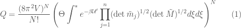
where  is the excess energy, basically the potential energy, including the quantum vibrational ground state energy, of the subsystem defined by a single solute molecule and
  solvent molecules,
  the overall volume of the system,
  the generalized internal coordinates of a single solute molecule with fixed rototranslational coordinates and
  the coordinates of the solvent molecules within the solute molecular volume. Moreover
  is the mass tensor of the
  solvent molecule,
  the mass tensor of the solute and
  a temperature dependent factor including the quantum corrections

with  and
and  the symmetry coefficient for the solute and the solvent respectively,
  and
and  the number of classical degrees of freedom in the solute and solvent molecules and
  and
and  the solvent and solute molecular quantum vibrational partition functions respectively. Finally the integral is taken within the solute molecular volume
  , and the star denotes an integration only over the accessible configurational space. From the previous equations it follows that the whole partition function can be obtained from the solute molecular partition function

where we used the approximation  . Hence, the whole thermodynamics is defined by
  as
as 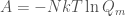 . This clearly means that if we want to describe the thermodynamics of the same system using the isobaric ensemble we must use a solute molecular isobaric partition function defined as
providing  (note that
  is an arbitrary volume constant necessary to make adimensional
  ). It is possible to show that

with  , the subscript
  indicating an average in the ensemble and
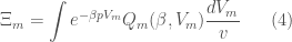
  . The ensemble average in Eq. 5 can be expressed as

where  is the enthalpy probability distribution function.
Instead of using a perturbation expansion, in the QGE theory, the free energy is obtained by modeling the distribution function and hence its moment generating function or Laplace transform, Eq. 6. For homogeneous fluid state systems, it was shown that a rather good model in the isobaric ensemble is the diverging Gamma state model for enthalpy fluctuations.
NOTE: The Gamma Distribution
The gamma distribution is a two-parameter family of continuous probability distributions. The exponential distribution, and chi-squared distribution are special cases of the gamma distribution.
For the two parameters  , it defined as
 for
for  and
and 
where $\Gamma(\alpha)$ is the gamma function

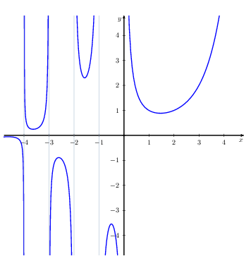
IN the following figure, the plot of the gamma distribution (left) for different value of and the  function are shown.
When we deal with a very complex system involving a macromolecule, it is likely that we need more sophisticated models. For the canonical ensemble, that the use of mixing distributions for Gamma state models provides a very powerful method to obtain more sophisticated and accurate models for fluid state systems. We can use a similar approach in the present case, assuming that the solute molecular configurational space of the internal coordinates can be partitioned into a set of  subspaces, each one defining a solute-solvent system exactly described by a “local” diverging Gamma state (note that the pure water thermodynamics is well described over a wide temperature range by a single diverging Gamma state). We can rewrite the total free energy change as
![\beta G(\beta) - \beta_0 G(\beta_0) = -N \ln \left\{ \sum_{i=1}^{L} \epsilon_i e^{- [n \Delta (\beta \mu_s) - \Delta (\beta \mu_i) ]} \right\}](https://s0.wp.com/latex.php?latex=%5Cbeta+G%28%5Cbeta%29+-+%5Cbeta_0+G%28%5Cbeta_0%29+%3D+-N+%5Cln+%5Cleft%5C%7B+%5Csum_%7Bi%3D1%7D%5E%7BL%7D+%5Cepsilon_i+e%5E%7B-+%5Bn+%5CDelta+%28%5Cbeta+%5Cmu_s%29+-+%5CDelta+%28%5Cbeta+%5Cmu_i%29+%5D%7D+%5Cright%5C%7D&bg=ffffff&fg=444444&s=0&c=20201002)

where  is the Gibbs free energy of the system defined by the solute molecular volume which contains solvent molecules and a single solute molecule in the
  th conformation (th subspace),
  is the chemical potential of the solvent and clearly
  is the chemical potential of the solute in the
  conformation. Finally,


with  , and
, and  the partition function corresponding to the ith conformation at . At high dilution the solvent molecular partial properties are identical to the pure solvent ones (hence independent of the solute). Within the assumption that each can be well modeled by a “local” diverging Gamma state, at infinite solute dilution we have

with  ,
,  and
and  the partial molecular enthalpy, heat capacity and entropy of the solute in the conformation at the reference temperature
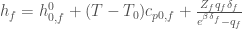
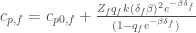
  . >From the other general equations of the diverging Gamma state properties we can also obtain all the other partial molecular properties of the solute, e.g. the enthalpy
  and heat capacity


where the zero subscript indicates the value at the reference temperature  . In the present case where we deal with complex macromolecules like proteins at fixed pressure, the summation in Eq. 1 is likely to involve a very large number of Gamma states corresponding to different protein configurational subspaces (conformations). Hence, in order to keep handable the mathematical derivations and especially the model application, we must use drastic simplifications. We will first assume that we can decompose the huge number of Gamma states into two subgroups: one associated with the folded state of the protein and one with the unfolded state. Moreover, we will assume also that within each subgroup the partial molecular heat capacity is the same for the different Gamma states and
  with
with  and
and  the overall “ground state” enthalpy (at ) and enthalpy gap of the subgroup. Hence, using the subscripts
  and
and  to define the folded and unfolded state properties respectively, we obtain


where  ,
,  ,
,  ,
,  are the total fractions and chemical potentials of the folded and unfolded subgroups and


From the previous equations we readily obtain the other partial molecular properties, i.e. enthalpy, entropy and heat capacity,


where obviously


are the corresponding partial molecular properties in the folded or unfolded state. Note that in the limit of a differential  and
and  a continuous Gamma states partition of the solute intramolecular phase space is involved.
For describing the state of complex systems, as biomacromolecules, the discrete-like diverging Gamma state partition seems to provide a better general description. The use of a discrete-like diverging Gamma states partition implies that the thermodynamics of a solvated macromolecule should be a complex mixture between a typical fluid state behavior and a discrete-like “energy” fluctuation. In order to proceed further we must model the discrete probability distribution  . A simple discrete distribution, which is phisically acceptable and proved to be succesfull to model quantum solid state, is the negative binomial distribution providing

where  and
and  are two pure numbers characteristic of the negative binomial distribution. With these last equations we can express the partial molecular properties of the folded and unfolded states as


and so


We can simplify further the model assuming that 
 and taking the reference temperature as the equilibrium temperature, i.e.,
  .
.
With these simplifications we obtain


which can be used to obtain the solute partial molecular properties, e.g., via Eq.~<a href=”#eqcv”>1</a> the partial molecular heat capacity.
NOT YET FINISHED!
BIBLIOGRAPHY
- Roccatano, A. Di Nola, A. Amadei. A theoretical model for the folding/unfolding thermodynamics of single-domain proteins, based on the quasi-Gaussian entropy theory. J. Phys. Chem. B, 108, 5756-5762 (2004).
- M.E.F Apol. The quasi-Gaussian entropy theory: Temperature dependence of thermodynamic properties using distribution functions. Ph.D. Thesis, Groningen (The Netherlands), 1997.
- A. Amadei. Theoretical models for fluid thermodynamics based on the quasi-Gaussian Entropy theory. Groningen (The Netherlands), Ph.D. Thesis, Groningen (The Netherlands), 1998.