“… Mitchell Feigenbaum was an unusual case. He had exactly one published article to his name, and he was working on nothing that seemed to have any particular promise. His hair was a ragged mane, sweeping back from his wide brow in the style of busts of German composers… At the age of twenty he had already become a savant among savants, an ad hoc consultant [at Los Alamos National Laboratory, USA] whom scientist would go to see about any expecially intractable problem.”
James Gleick, Chaos: the amazing science of the unpredectable.
This year, on June 30th 2019, Mitchell J. Feigenbaum died at the age of 74. Feigenbaum was an American mathematician that became famous with the discovery of the universal constants that bear his name. In the middle of the ’80, reading Le Scienze magazine (the Italian edition of Scientific American) I got to know of the contribution to the chaos theory of this charismatic mathematician. In particular, I was delighted by reading the Douglas Hofstadter’s article in the rubric “Temi Metamagici” ( Methamagical themes) (Scientific American, November 1981). The article explained the emergence of the chaos in the iteration map of the logistic equation, the same equation deeply studied by Feigenbaum. The full story about the Mitchell Feigenbaum and his discovery of his universal constants is delightly narrated in the beautiful book Chaos:the amazing science of the unpredectable by J. Gleick [1]. Here it is just another small extract:
“… in the summer of 1975, at a gathering in Aspen, Colorado, he heard Steve Smale [another key mathematicial in the developing of the chaos theory, NDA] talk about some of the mathematical qualities of the same quadratic difference equation [the same studied by Robert May, NDA]. Smale seemed to think that there were some interesting open questions about the exact point at which the mapping changes from periodic to chaotic. As always, Smale had a sharp instinct for questions worth exploring. Feigenbaum decided to look into it once more.”[1]
To better understand the contribution of Feigenbaum to the chaos theory, we need some background information. The story begin with a 1976 article on Nature [2] by Lord Robert May of Oxford that reported a curious behaviour in the iteration map of the logistic equation. Prof. May was a famous applied mathematics that give key contributions to the theoretical ecology. In his Nature paper, he analyzed the mathematical behaviour of a population of insect described by the Velhulst model of population grow. The mathematician Pierre François Verhulst studied this model in the first half of the 1800 when he was studying population models. He found out that a population cannot growth indefinitively but it is limited by the availability of food. To explain mathematically such process, he used the following differential equation (DE) that consist in the classic law of exponential law with in addition a non-linear term that limit the grow of the population:

The parameter $lambda$ control the spped at which the population grow. May noticed that increasing the value of $lambda$ the behaviour of the DE undergoes a process of period bifurcation that bring to the emergence of a chaotic behaviour.
Before continuing I will make now a short detour to explain the title of this article. After reading the Hofstadter’s article, in the verge of my BASIC programming fascination, I wrote a program in MSX BASIC language to reproduce the illustration in the article. In my retro-nostalgic archaeology survey, I managed to recover this program from an old magnetic tape. To retrieve the listing of these programs, I have used the open software MSX emulator OpenMSX (https://openmsx.org) but editing the application using this emulator is not in my retro programming intentions! Fortunately, the MSX Basic is Microsoft product, and as such, it is indeed very similar to the other Basic from the same company. I found two great programs that can nicely run native Quick Basic BASIC program on my MacBook and they considerably helped me in this enterprise. One is the PC-BASIC, a Python-based interpreter, and the other the QB64, a QuickBasic compiler. The first application using Python run the code quite slowly so it is not very convenient for calculation intensive program. The second one, as it transforms the BASIC program code in Basic to C++ language, and then compile it. Therefore, it is much faster and useful for producing usable programs for modern computers. Hence, I adapted with little adjustments the orginal MS BASIC codes to run them on the QB64 compiler. I also take the change to clean up a bit the code and add some new feature that will be useful to illustrate this blog. The source code of the program is reported in the Appendix.
The study of a DE can be performed by using a map of it. A map is a recursive representation of the DE solution. In the case of the logistic equation the map is given by the relation

A map is a discrete representation of the DE that use the result on the right side of the DE for a certain value of $x_i$ to calculate its next value 


 .
.For 

 .
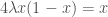
.When the value of 
 .
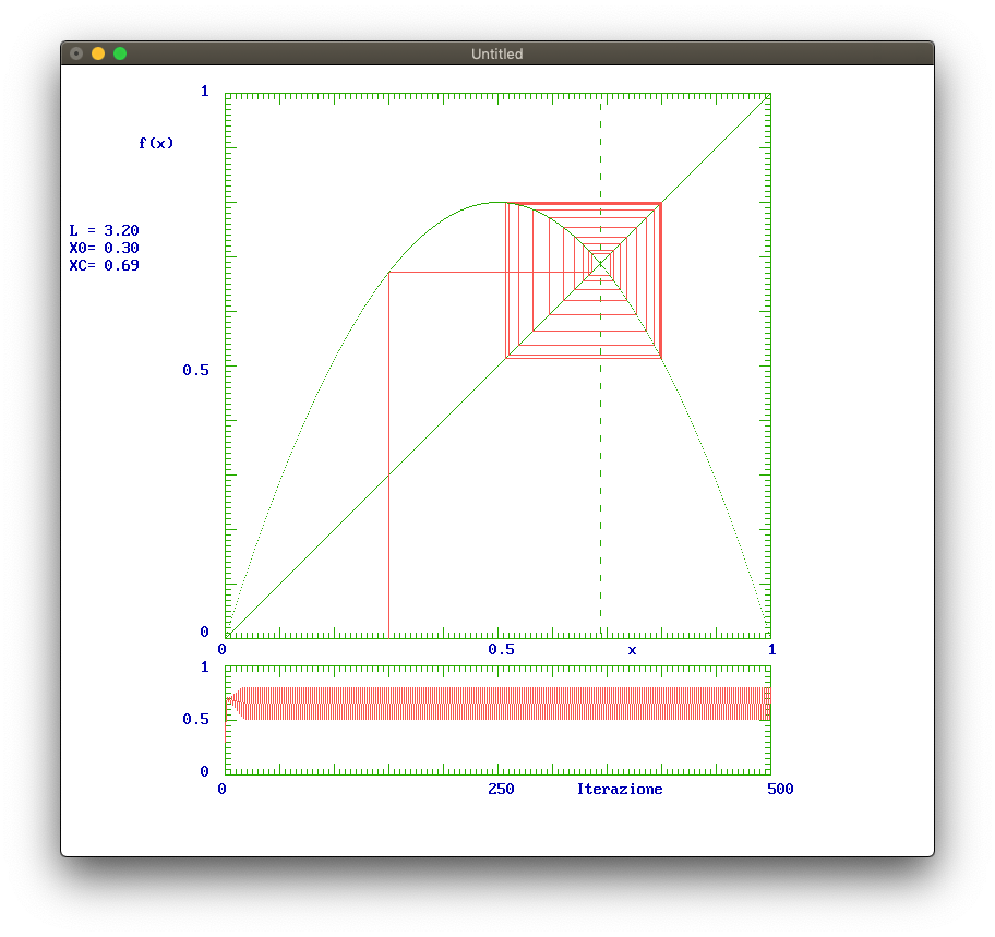
.To better understand what it is happening, we need to look to the position of the fixed points of the second iterate function (indicated as 


 with
with  the logistic equation and
  .
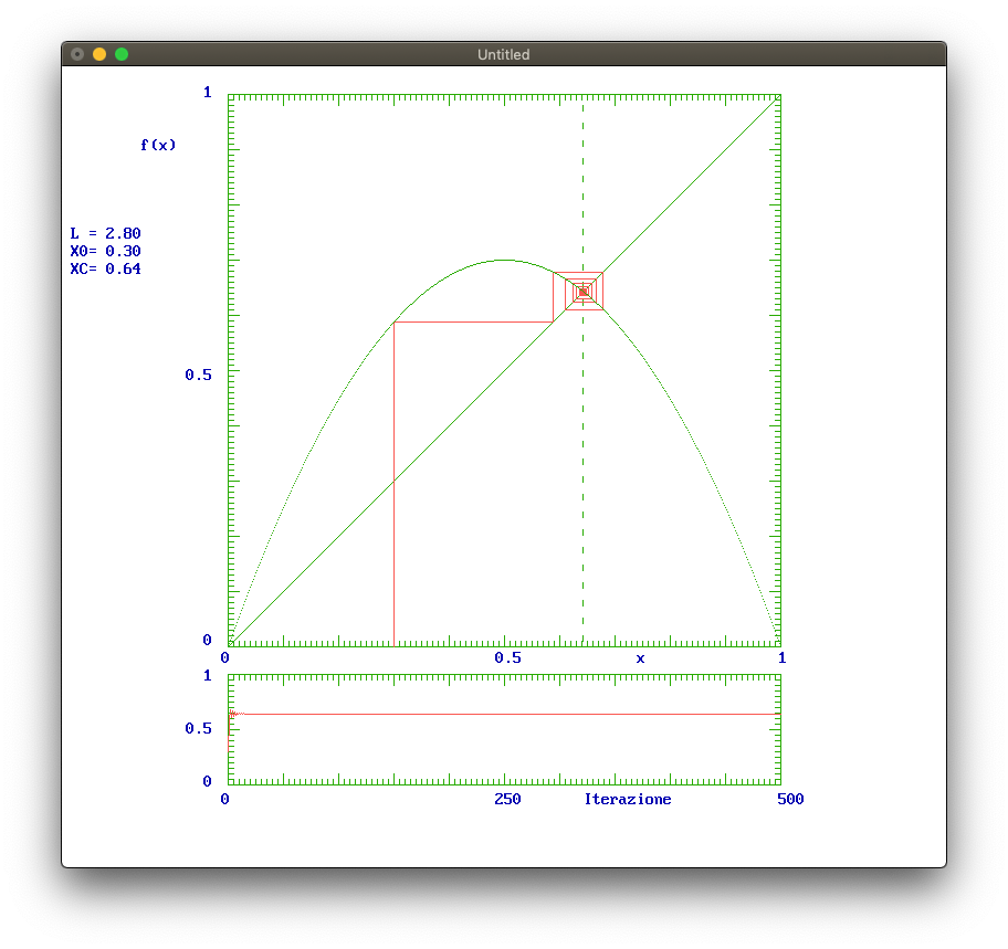
.By further increasing the value of 


 .
.The doubling period behaviour continue until a value 
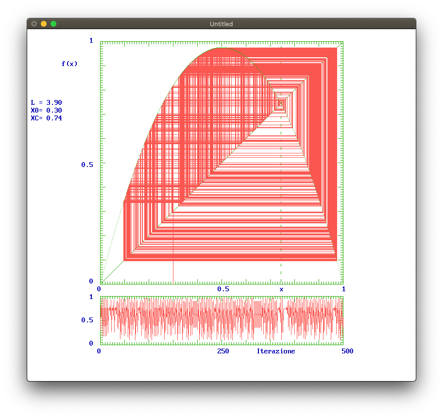
The diagram shown in Figure 7 (sometime called Figenbaum plot) represents the value of the iterated logistic equation versus the parameter 

After the article of May, other experts in dynamical systems started to study the iterate of quadratic functions. They were particulary puzzled by the transition from the period doubling to the chaotic regime. As storytellered by Gleick in his book (see the citation above) it was in a seminar by the famous mathematician Steven Smale that Figenbaum got the inspiration for starting his investigation on this problem. In his early research, Figenbaum used a card programmable HP 65 pocket calculator to evaluate the result of the iterations of the function 


Therefore, as first guess, the ratio
$\latex \delta=\frac{\delta_k}{\delta_{k+1}}$
should give the relation for a geometric decrease of distances. In reality, it is only an approximation as the distance change from bifurcation to bifurcation [6]. However, in the limit of large value of k this relation is correct

The BASIC program reported in the appendix implement an algorithm for the calculation of the approximate value of the Figenbaum constant (see [6] for the description).
Figenbaum also found out that differently by the value of the Figenbaum point, that dipends by the scalling factor, the Figenbaum constant retain the same value for different type of interated functions [4,5] (as for example the exponential function reported in Figure 9).

These findings, tough very interesting, would remain a mathematics curiosity if few years after their publication, ana italian physicist studying the stability of the laser light come across with a phenomena involving period-doubling. This discovery was followed by many other involved other dynamics system, and all of them shared a same Universal constant: the Figenbaum constant.
The reader interested to read a full story about M. J. Fiegenbaum’s live and scientific work can find a wonderful article signed by Stephen Wolfram on his blog [7].
BIBLIOGRAPHY
- J. Gleick. Chaos: Making a New Science.
- May, Robert M. (1976). “Simple mathematical models with very complicated dynamics”. Nature. 261 (5560): 459–467.
- Feigenbaum, M.J., 1978. Quantitative universality for a class of nonlinear transformations. Journal of statistical physics, 19(1), pp.25-52.
- Feigenbaum, M. J. “The Universal Metric Properties of Nonlinear Transformations.” J. Stat. Phys.21, 669-706, 1979.
- Feigenbaum, M.J., 1983. Universal behavior in nonlinear systems. Physica D: Nonlinear Phenomena, 7(1-3), pp.16-39.
- Peitgen, H.O., Jürgens, H. and Saupe, D., 2006. Chaos and fractals: new frontiers of science. Springer Science & Business Media. This book is an excellent introduction to this topics (in particular read the chapter 1, 10 and 11).
- Stephen Wolfram”Mitchell Feigenbaum (1944‑2019), 4.66920160910299067185320382…” : https://writings.stephenwolfram.com/2019/07/mitchell-feigenbaum-1944-2019-4-66920160910299067185320382 (last accessed 28/12/2019)
APPENDIX
This is the program in BASIC language that was used to generate the picture in this article. The program is provided as it is and the author decline responsabilities for bugs and/or incorrect results that it may produce (see About). You are welcome to improve it and if you do so please send me back your updated version!
'================================================================
' PROGRAMMA  : MAPPE_LOGISTICHE.BAS
' DESCRIZIONE: QUESTO PROGRAMMA CALCOLA LE PROPRIETA' DINAMICHE
'              DELLA FUNZIONE LOGISTICA
'              PER MAGGIORI INFORMAZIONE SI CONSULTI
'              L'ARTICOLO DI David HOFSTATDER
'              "Strani attarttori:schemi matematici collocati fra
'               l'ordine e il caos' APPARSO NELLA RUBRICA
'              "TEMI METAMAGICI" NEL NUMERO 162 (Febbraio 1982)
'              DI LE SCIENZE.
' AUTORE     : D. ROCCATANO
' CREATO NEL : 1985
'================================================================

DIM SHARED XI, CI, CF, NITER, H AS INTEGER
DIM SHARED G, L AS DOUBLE

CF = 2
CI = 12
G = 1 / 500
NITER = 500

SCREEN _NEWIMAGE(800, 725, 256)
'WIDTH 80
CLS
COLOR 1, 15
OUT &H3C8, 0
OUT &H3C9, 63
OUT &H3C9, 63
OUT &H3C9, 63

'   ====  MENU DEL PROGRAMMA  =====
LOCATE 5, 5: PRINT "STUDIO DELLE ITERATE DELLA FUNZIONE LOGISTICA"
LOCATE 10, 10: PRINT "[1] STUDIO NELLE FUNZIONI ITERATE"
LOCATE 11, 10: PRINT "[2] STUDIO DELLA FUNZIONE LOGISTICA vs NUMERO D'ITERAZIONI"
LOCATE 12, 10: PRINT "[3] STUDIO DELLA FUNZIONE LOGISTICA vs PARAMETRO LAMBDA"
LOCATE 13, 10: PRINT "[4] CALCOLO DELLA COSTANTE DI FIGENBAUM "
LOCATE 14, 10: PRINT "[5] ESCI "
LOCATE 16, 12: INPUT "Scegli una opzione: "; H
SELECT CASE H
    CASE 1
        MENU1 H
    CASE 2
        TRAJ H
    CASE 3
        BIFORC
    CASE 4
        FIGEN
    CASE 5
        END
END SELECT
RUN
END
'   ====  PARTE 1 =====
SUB MENU1 (H)
    SHARED CI, CF, NITER
    SHARED G, L
    WHILE HH <> 5
        CLS
        LOCATE 5, 3: PRINT "VISUALIZZAZIONE PUNTI STAZIONARI DI FUNZIONI LOGISTICHE"
        LOCATE 8, 10: PRINT "1] x=f(x)=L*x*(1-x)"
        LOCATE 9, 10: PRINT "2] x=f(f(x))"
        LOCATE 10, 10: PRINT "3] x=f(f(f(x)))"
        LOCATE 11, 10: PRINT "4] x=f(f(f(f(x))))"
        LOCATE 12, 10: PRINT "5] RITORNA AL MENU PRINCIPALE"
        LOCATE 14, 12: INPUT "Scegli una opzione: "; HH
        IF HH = 5 THEN EXIT WHILE
        LOCATE 16, 14: INPUT "Inserisci il valore di lambda (L)"; L
        PRINT
        LOCATE 18, 14: INPUT "Inserisci il valore iniziale di x"; XS
        '
        ' Disegna il grafico
        '
        FRAME H
        LOCATE 34, 66: PRINT "x"
        LOCATE 34, 19: PRINT "0"
        LOCATE 34, 82: PRINT "1"
        LOCATE 34, 50: PRINT "0.5"
        LOCATE 10, 2: PRINT USING "L = #.##"; L
        LOCATE 11, 2: PRINT USING "X0= #.##"; XS

        '
        ' Vai all subroutine di rappresentatione della funzione
        '
        SELECT CASE HH
            CASE 1
                ITER1 XS, L
            CASE 2
                ITER2 XS, L
            CASE 3
                ITER3 XS, L
            CASE 4
                ITER4 XS, L
        END SELECT
    WEND
END SUB
'      SUBROUTINES
SUB ITER1 (XS, L)
    '   ---- ITERAZIONE FUNZIONE N. 1 ---
    SHARED XI, CI, CF, NITER
    LOCATE 5, 10: PRINT "f(x)"
    ' TRACCIA LA POSIZIONE DEL PUNTI CRITICI
    XCP = 1 - 1 / L
    LOCATE 12, 2: PRINT USING "XC= #.##"; XCP
    LINE (FNX(XCP), 25)-(FNX(XCP), 525), 2, , 63
    FUNC1 G, L
    X = XS
    Y = L * X * (1 - X)
    LINE (FNX(X), 525)-(FNX(X), FNY(Y)), CI
    FOR K = 1 TO NITER
        Y = FNF(X, L)
        N = 500 * Y + XI
        LINE (150 + (K - 1), 650 - 100 * X)-(150 + K, 650 - 100 * Y), CI
        LINE (FNX(X), FNY(Y))-(N, FNY(Y)), CI
        M = FNF(Y, L)
        LINE (N, FNY(Y))-(N, 525 - 500 * M), CI
        X = Y
    NEXT K
    FUNC1 G, L

    K$ = INPUT$(1)
END SUB
SUB ITER2 (XS, L)
    SHARED XI, CI, CF, NITER
    '   ---- ITERAZIONE FUNZIONE N. 2 ---
    ' TRACCIA LA POSIZIONE DEL PUNTI CRITICI

    XCP = 1 - 1 / L
    IF (L >= 3) THEN
        XCP1 = ((L + 1) + SQR((L + 1) * (L - 3))) / (2 * L)
        XCP2 = ((L + 1) - SQR((L + 1) * (L - 3))) / (2 * L)
        LOCATE 13, 2: PRINT USING "XC1= #.##"; XCP1
        LOCATE 14, 2: PRINT USING "XC=2 #.##"; XCP2
        LINE (FNX(XCP1), 25)-(FNX(XCP1), 525), 2, , 63
        LINE (FNX(XCP2), 25)-(FNX(XCP2), 525), 2, , 63
    END IF
    LOCATE 12, 2: PRINT USING "X*= #.##"; XCP
    LOCATE 13, 2: PRINT USING "XR= #.##"; XCP1
    LOCATE 14, 2: PRINT USING "XL= #.##"; XCP2

    LINE (FNX(XCP), 25)-(FNX(XCP), 525), 2, , 63
    FUNC2 G, L
    LOCATE 5, 10: PRINT "f(f(x))"
    X = XS
    S = FNF(X, L)
    Y = FNF(S, L)
    LINE (FNX(X), 525)-(FNX(X), FNY(Y)), CI
    FOR K = 1 TO NITER
        S = FNF(X, L)
        Y = FNF(S, L)
        N = 500 * Y + XI
        LINE (FNX(X), FNY(Y))-(N, FNY(Y)), CI
        S = FNF(Y, L)
        M = FNF(S, L)
        LINE (N, FNY(Y))-(N, 525 - 500 * M), CI
        X = Y
    NEXT K
    FOR K = 1 TO NITER
        Y = FNF(X, L)
        N = 500 * Y + XI
        LINE (150 + (K - 1), 650 - 100 * X)-(150 + K, 650 - 100 * Y), CI
        LINE (FNX(X), FNY(Y))-(N, FNY(Y)), CI
        M = FNF(Y, L)
        LINE (N, FNY(Y))-(N, 525 - 500 * M), CI
        X = Y
    NEXT K

    FUNC2 G, L
    K$ = INPUT$(1)
END SUB
SUB ITER3 (XS, L)
    '   ---- ITERAZIONE FUNZIONE N. 3 ---
    SHARED XI, CI, CF, NITER
    FUNC3 G, L
    LOCATE 5, 9: PRINT "f(f(f(x)))"
    X = XS
    S = FNF(X, L)
    V = FNF(S, L)
    Y = FNF(V, L)
    LINE (FNX(X), 525)-(FNX(X), FNY(Y)), CI
    FOR K = 0 TO NITER
        S = FNF(X, L)
        V = FNF(S, L)
        Y = FNF(V, L)
        N = 500 * Y + XI
        LINE (FNX(X), FNY(Y))-(N, FNY(Y)), CI
        S = FNF(Y, L)
        P = FNF(S, L)
        M = FNF(P, L)
        LINE (N, FNY(Y))-(N, 525 - 500 * M), CI
        X = Y
    NEXT K
    FOR K = 1 TO NITER
        Y = FNF(X, L)
        N = 500 * Y + XI
        LINE (150 + (K - 1), 650 - 100 * X)-(150 + K, 650 - 100 * Y), CI
        LINE (FNX(X), FNY(Y))-(N, FNY(Y)), CI
        M = FNF(Y, L)
        LINE (N, FNY(Y))-(N, 525 - 500 * M), CI
        X = Y
    NEXT K

    FUNC3 G, L
    K$ = INPUT$(1)
END SUB
SUB ITER4 (XS, L)
    SHARED XI, CI, CF, NITER
    '   ---- ITERAZIONE FUNZIONE N. 4 ---
    FUNC4 G, L
    LOCATE 5, 5: PRINT "f(f(f(f(x))))"
    X = XS
    K = FNF(X, L)
    V = FNF(K, L)
    F = FNF(V, L)
    Y = FNF(F, L)
    LINE (FNX(X), 525)-(FNX(X), FNY(Y)), CI
    FOR K = 1 TO NITER
        K = FNF(X, L)
        V = FNF(K, L)
        F = FNF(V, L)
        Y = FNF(F, L)
        N = 500 * Y + 150
        LINE (FNX(X), FNY(Y))-(N, FNY(Y)), CI
        S = FNF(Y, L)
        P = FNF(S, L)
        T = FNF(P, L)
        M = FNF(T, L)
        LINE (N, FNY(Y))-(N, 525 - 500 * M), CI
        X = Y
    NEXT K
    FOR K = 1 TO NITER
        Y = FNF(X, L)
        N = 500 * Y + XI
        LINE (150 + (K - 1), 650 - 100 * X)-(150 + K, 650 - 100 * Y), CI
        LINE (FNX(X), FNY(Y))-(N, FNY(Y)), CI
        M = FNF(Y, L)
        LINE (N, FNY(Y))-(N, 525 - 500 * M), CI
        X = Y
    NEXT K
    FUNC4 G, L
    K$ = INPUT$(1)
END SUB

SUB FRAME (H)
    '   DRAW THE GRAPH FRAME
    SHARED XI, CF
    CLS
    XI = 150
    XF = XI + 500
    '   DRAW GRAPH FRAME
    LINE (XI, 25)-(XF, 525), CF, B
    IF H < 2 THEN LINE (XI, 525)-(XF, 25), CF
    '   DRAW x-ticks
    FOR I = XI TO XF STEP 5
        LINE (I, 25)-(I, 25 + 5), CF
        LINE (I, 525)-(I, 525 - 5), CF
    NEXT
    FOR I = XI TO XF STEP 50
        LINE (I, 25)-(I, 25 + 10), CF
        LINE (I, 525)-(I, 525 - 10), CF
    NEXT
    '   DRAW y-tics
    FOR I = 525 TO 25 STEP -5
        LINE (XI, I)-(XI + 5, I), CF
        LINE (XF, I)-(XF - 5, I), CF
    NEXT
    FOR I = 525 TO 25 STEP -50
        LINE (XI, I)-(XI + 10, I), CF
        LINE (XF, I)-(XF - 10, I), CF
    NEXT
    LOCATE 2, 17: PRINT "1"
    LOCATE 18, 15: PRINT "0.5"
    LOCATE 33, 17: PRINT "0"
    IF H = 1 THEN
        ' Disegna il grafico della funzione rispetto alle iterazioni
        LINE (XI, 550)-(XF, 650), CF, B
        LOCATE 35, 17: PRINT "1"
        LOCATE 38, 15: PRINT "0.5"
        LOCATE 41, 17: PRINT "0"
        LOCATE 42, 19: PRINT "0"
        LOCATE 42, 82: PRINT "500"
        LOCATE 42, 50: PRINT "250"
        LOCATE 42, 60: PRINT "Iterazione"
        '   DRAW x-ticks
        FOR I = XI TO XF STEP 5
            LINE (I, 550)-(I, 550 + 5), CF
            LINE (I, 650)-(I, 650 - 5), CF
        NEXT
        FOR I = XI TO XF STEP 50
            LINE (I, 550)-(I, 550 + 10), CF
            LINE (I, 650)-(I, 650 - 10), CF
        NEXT
        '   DRAW y-tics
        FOR I = 650 TO 550 STEP -5
            LINE (XI, I)-(XI + 5, I), CF
            LINE (XF, I)-(XF - 5, I), CF
        NEXT
        FOR I = 650 TO 550 STEP -50
            LINE (XI, I)-(XI + 10, I), CF
            LINE (XF, I)-(XF - 10, I), CF
        NEXT
    END IF
END SUB

SUB TRAJ (H)
    SHARED CI, XI
    '   ==== CALCOLO 2  ====
    '   ==== Traiettorie della funzione ====
    LOCATE 18, 14: INPUT "Inserisci il valore iniziale di lambda L"; L
    PRINT
    LOCATE 19, 14: INPUT "  Inserisci il valore iniziale di x"; XS
    FRAME H
    LOCATE 1, 5: PRINT "GRAFICO DELLA FUNZIONE LOGISTICA f(x)=L*x*(1-x) VERSO IL NUMERO DI ITERAZIONI"
    LOCATE 5, 10: PRINT "f(x)"
    LOCATE 34, 66: PRINT "Iterazione"
    LOCATE 34, 19: PRINT "0"
    LOCATE 34, 82: PRINT "500"
    LOCATE 34, 50: PRINT "250"
    LOCATE 15, 2: PRINT USING "LAMBDA : ##.###"; L
    LOCATE 16, 2: PRINT USING "X0: ##.###"; XS

    X = XS
    '   === ELIMIINATE TRANSIENTS ===
    FOR I = 1 TO 100
        X = L * X * (1 - X)
    NEXT I
    XO = X
    FOR I = 2 TO 499
        X = L * X * (1 - X)
        LINE (150 + (I - 1), 525 - 500 * XO)-(150 + I, 525 - 500 * X), CI
        XO = X
    NEXT I
    K$ = INPUT$(1)
END SUB
SUB BIFORC
    '   ==== CALCOLO 3  ====
    '   ==== GRAFICO DELLE BIFORCAZIONI
    WHILE HH <> 5
        CLS
        LOCATE 5, 3: PRINT "VISUALIZZAZIONE PUNTI STAZIONARI DI FUNZIONI LOGISTICHE"
        LOCATE 8, 10: PRINT "1] f(x)=f(x)=L*x*(1-x)"
        LOCATE 9, 10: PRINT "2] f(x)=L*X     IF X< 1/2"
        LOCATE 10, 10: PRINT "   f(x)=L*(1-X) IF X> 1/2"
        LOCATE 11, 10: PRINT "3] f(x)=x*exp(l*(1-x))"
        LOCATE 12, 10: PRINT "4] RITORNA AL MENU PRINCIPALE"
        LOCATE 14, 12: INPUT "Scegli una opzione: "; HH
        IF HH = 4 THEN EXIT WHILE
        IF HH > 0 AND HH < 5 THEN
            LOCATE 18, 14: INPUT "Inserisci il valore iniziale di L:"; L0
            LOCATE 19, 14: INPUT "Inserisci il valore finale di L  :"; LF
            LOCATE 20, 14: INPUT "Inserisci numero d'iterazioni    :"; NITER
            FRAME H
            LOCATE 5, 15: PRINT "f(x)"
            LOCATE 41, 22: PRINT USING "NUMERO DI ITERAZIONI= #####"; NITER
            LOCATE 34, 66: PRINT "L"
            LOCATE 34, 19: PRINT L0
            LOCATE 34, 82: PRINT LF
            LOCATE 34, 50: PRINT L0 + (LF - L0) / 2
            SELECT CASE HH
                CASE 1
                    LOGISTIC L0, LF, NITER
                CASE 2
                    CUSPID L0, LF, NITER
                CASE 3
                    EXPON L0, LF, NITER
            END SELECT
        END IF
    WEND
END SUB

SUB LOGISTIC (L0, LF, NITER)
    LOCATE 38, 22: PRINT "f(x)=f(x)=L*x*(1-x)"
    L0 = L0
    LF = LF
    XS = 0.5
    S = (LF - L0) / 500
    DD = 0
    FOR L = L0 TO LF STEP S
        X = XS
        FOR I = 1 TO 100
            X = L * X * (1 - X)
        NEXT I
        FOR I = 1 TO NITER
            X = L * X * (1 - X)
            IF X >= 0 AND X <= 1 THEN
                PSET (150 + (L - L0) / S, 525 - 500 * X), CI
            END IF
        NEXT I
    NEXT L
    K$ = INPUT$(1)
END SUB

SUB CUSPID (L0, LF, NITER)
    LOCATE 38, 22: PRINT "2] f(x)=L*X     IF X< 1/2"
    LOCATE 39, 22: PRINT "   f(x)=L*(1-X) IF X> 1/2"

    XS = 0.3
    S = (LF - L0) / 500
    DD = 0
    FOR L = L0 TO LF STEP S
        X = XS
        FOR I = 1 TO 100
            IF X < 0.5 THEN
                X = L * X
            ELSE
                X = L * (1 - X)
            END IF
        NEXT I
        FOR I = 1 TO NITER
            IF X < 0.5 THEN
                X = L * X
            ELSE
                X = L * (1 - X)
            END IF
            IF X >= 0 AND X <= 1 THEN
                PSET (150 + (L - L0) / S, 525 - 500 * X), CI
            END IF
        NEXT I
    NEXT L
    K$ = INPUT$(1)
END SUB

SUB EXPON (L0, LF, NITER)
    LOCATE 38, 22: PRINT "3] f(x)=x*exp(l*(1-x))"

    XS = 0.3
    S = (LF - L0) / 500
    DD = 0
    FOR L = L0 TO LF STEP S
        X = XS
        FOR I = 1 TO 100
            X = X * EXP(L * (1 - X))
        NEXT I
        FOR I = 1 TO NITER
            X = X * EXP(L * (1 - X))
            IF X >= 0 AND X <= 1 THEN
                PSET (150 + (L - L0) / S, 525 - 500 * X), CI
            END IF
        NEXT I
    NEXT L
    K$ = INPUT$(1)
END SUB


SUB FUNC1 (G, L) '   === DISEGNA LA FUNZIONE 1 ===
    SHARED CF
    FOR X = 0 TO 1 STEP G
        Y = FNF(X, L)
        PSET (FNX(X), FNY(Y)), CF
    NEXT
END SUB
SUB FUNC2 (G, L) '   ==== DISEGNA LA FUNCTIONE 2 ===
    SHARED CF
    FOR X = 0 TO 1 STEP G
        K = FNF(X, L)
        Y = FNF(K, L)
        PSET (FNX(X), FNY(Y)), CF
    NEXT
END SUB
SUB FUNC3 (G, L) '   === DISEGNA LA FUNCTIONE 3 ====
    SHARED CF
    FOR X = 0 TO 1 STEP G
        K = FNF(X, L)
        V = FNF(K, L)
        Y = FNF(V, L)
        PSET (FNX(X), FNY(Y)), CF
    NEXT
END SUB
SUB FUNC4 (G, L) '   === DISEGNA LA FUNCTIONE 4 ====
    SHARED CF
    FOR X = 0 TO 1 STEP G
        K = FNF(X, L)
        V = FNF(K, L)
        F = FNF(V, L)
        Y = FNF(F, L)
        PSET (FNX(X), FNY(Y)), CF
    NEXT
END SUB
SUB FIGEN '   CALCOLO DELLA COSTANTE UNIVERSALE DI FEIGENBAUM
    '
    '
    A1 = 1
    A2 = 0
    D1 = 3.2
    MAXI = 8
    MAXJ = 10
    PRINT " i       Figenbaum Delta"
    FOR I = 2 TO MAXI STEP 1
        A = A1 + (A1 - A2) / D1
        FOR J = 1 TO MAXJ STEP 1
            X = 0
            Y = 0
            FOR K = 1 TO 2 ^ I STEP 1
                Y = 1.0 - 2.0 * Y * X
                X = A - X * X
            NEXT K
            A = A - X / Y
        NEXT J
        D = (A1 - A2) / (A - A1)
        PRINT I, D
        D1 = D
        A2 = A1
        A1 = A
    NEXT I
    PRINT "VALORE FINALE: ", D
    K$ = INPUT$(1)
END SUB

FUNCTION FNX (X)
    FNX = 500 * X + 150
END FUNCTION
FUNCTION FNY (Y)
    FNY = 525 - 500 * Y
END FUNCTION
FUNCTION FNF (X, L)
    FNF = L * X * (1 - X)
END FUNCTION

