This article was inspired by the beautiful 2016 movie Hidden Figures (based on the book of the same name by M. L. Shetterley) which tell the dramatic story of three talented black women scientist that worked as “human computers” for NASA in 1961 for the Mercury project.

In the movie, the mathematician Creola Katherine Johnson (or Globe) (interpreted by Taraji P. Henson), had a brilliant intuition on how to numerically solve the complex problem to find the transfer trajectory for the reentry into the Earth atmosphere of the Friendship 7 capsule with the astronaut John Glenn on board. In the particular scene, she was standing together with other engineers and the director of the Langley Research Center (a fictional character interpreted by Kevin Coster) in front of the vast blackboard looking to graph and equations when she says that the solution might be in the “old math” and she runs to take an old book from a bookshelf with the description of the Euler method [UPDATE, May 2022: I just come across another excellent youtube video by the Tibees about the mathematical work of K. Johnson at NASA, and at the end of the video she reveal that the book shown in the movie is the classic H Margenau & G. M Murphy, The Mathematics of Physics and Chemistry. Published by Van Nostrand, 1956]. The scene is also nicely described in the youtube video lesson by Prof. Alan Garfinkel of the UCLA. A detailed description of the numerical solution based on the original derivation of K. Johnson is in the Wolfram blog website.
Katherine Globe was using for these complex calculation her brilliant brain with the support of a mechanical calculator (the Friden STW-10, in the movie, this machine is visible in different scenes). In a scene of the film, she revealed that her typical computing performance was of 10000 calculations per day and probably for calculations, she was not referring to single arithmetic operations! These exceptional mathematical skills have given a significative contribution at the beginning of the American space program, but it became insufficient to handle the more complex mathematics necessary to land the man on the Moon, and the other fantastic NASA achievements.
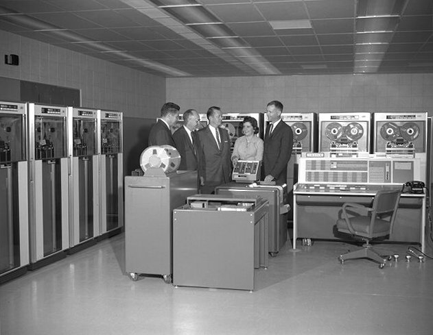
Therefore, at the end of the movie, it is shown that the Langley Research Center to keep pace with the progress of the technology the acquire one of just developed electronic computer: the IBM 7090. This computer was one of IBM’s first transistor-based computers specifically designed for the scientific computing that NASA needed for the Mercury and Gemini space missions. The processing speed of this computer was in the range of 100-200 Kflops/s with costs of millions of dollars, and definitively not easily transportable! Today, the smartphone in our pocket is easily tens of thousand times more powerful and less expensive!
Euler’s Method
Going back to the Euler method, let now see how it can be used to calculate trajectories of satellites by numerically integrating the law of gravity.
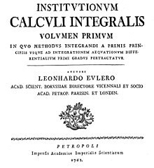
Leonhard Euler (1707-1783) was a genius polymath Swiss scientist and one of the most prolific mathematicians in history. To date, his complete opera, accounting thousand of papers written in Latin is yet not completely translated. The method to calculate approximately the solution of ordinary differential equations was reported in the book Institutionum calculi integralis (Foundations of Integral Calculus) published in 1768.
An ordinary differential equation (ODE) is an algebraic expression that put in relation the derivative of a dependent variable, with respect an independent one, to a function of both variables. For example in the differential equation

with 


Most problems in physics and engineering appear in the form of ordinary differential equations. For example, the motion of a particle is described by Newton’s equations, which is a second-order ordinary differential equation involving at least a second-order derivative in time, and the motion of a quantum particle is described by the Schrodinger equation, which is a partial differential equation involving a first-order partial derivative in time and second-order partial derivatives in coordinates.
The Initial-Value problem
An initial-value problem consists in the solution of (systems) DE’s describing dynamical systems as, for example, the motion of the Moon, Earth, and the Sun, the dynamics of a rocket, or the propagation of ocean waves, given the initial position and velocities of the system components. Many DE’s can be solved using integration methods of Calculus. However, it is usually hard if not impossible, to find an analytical solution. Euler was well aware of this difficulty and gave the most straightforward method for approximating a solution that brings his name.
A straightforward system is a particle of mass m moving in one dimension along the x-axis under an elastic force f(x). In this case, the Newton’s equation that governs the dynamics of the system is given by

where a and v are the acceleration and velocity of the particle, respectively, and t is the time. If we divide the time into small, equal intervals h = ti +1− ti, elementary physics tell us that the velocity at time 
![[t_i,t_{i+1}],](https://s0.wp.com/latex.php?latex=%5Bt_i%2Ct_%7Bi%2B1%7D%5D%2C&bg=ffffff&fg=444444&s=0&c=20201002)

the corresponding acceleration is approximately given by the average acceleration in the same time interval,

as long as τ is small enough. The simplest algorithm for finding the position and velocity of the particle at time ti+1from the corresponding quantities at time ti is obtained after combining the previous equations, and we have
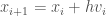

where 


Note that the above way of constructing an algorithm is not limited to one-dimensional or single-particle problems. In fact, we can immediately generalize this algorithm to two-dimensional and three-dimensional problems, or to the problems involving more than one particle, such as the motion of a projectile or a system of three charged particles. The generalized version of the above algorithm is

where R = (r1,r2,…,rn) is the position vector of all the n particles in the system; V = (v1,v2,…,vn)\ and A = (a1,a2,…,an), with aj= fj/mj for j = 1, 2, . . . , n, are the corresponding velocity and acceleration vectors, respectively. I will come back in another post about the numerical solution of DE systems.
The Euler’s method is based on the Taylor series representation of the DE solution. You can find more about Taylor series in another post, here we just recall the Taylor theorem
If 


The first sum on the right side of the equation is called the Taylor Polynomial of degree n and may be used to approximate

The Euler method is based on the first order Taylor polynomial approximation (


as 

with 


Therefore it is possible in principle to increase the accuracy of the numerical solution by descreasing the value of the increment h but paying the price of increase the number of steps required to reach the maximum value of t.
We can use a simple program in awk language to study the effect of the step size, h, on the accuracy of the solution of the ODE in (1). Given the initial conditions 


#======================================================================
#
#  NAME:  Euler.awk
#
#======================================================================
#  DESCRIPTION: Test the effect of the time step on the numerical
#               integration of the DE y'=cos(t) using the Euler method
#
#======================================================================
#  DEVELOPED USING: gawk
#  REQU. FUNCTIONS:
#======================================================================
# Author:        Danilo Roccatano
# Version:       1.0
# Copyright (C): 2019 Danilo Roccatano
#======================================================================
#

function f(t) {
    return cos(t)
}

BEGIN {
# Set the time steps to test
    h[0]= 0.005
    h[1]= 0.01
    h[2]= 0.05
    h[3]= 0.075
    h[4]= 0.1
    h[5]= 0.5
    h[6]= 1.0
# Set the end value of the integration interval in (radiants)
    T=1
# calculate the analytical solution a T
    cval=sin(T)
    printf "%8.3f \n",sin(1)
    for (j=0;j<7;j++) {
        hh=h[j]
        t=0
        N=T/hh
        y=0
        for (i=0;i<N;i++) {
            t=t+hh
            y=y+f(t)*hh
        }
        diff = cval-y
        printf "%d %8.3f %3d %8.3f (%8.3f) \n",j+1,hh,N,y,diff
    }
    printf "\n"

}
The results are listed in the following table. By increasing the time step the solution become more unstable giving larger and larger deviations from the correct value. The method used in the script is called forward Euler method and it belong to a class of method called explicit integration methods.
| # | TIme step | N. steps | Value | |Difference|* |
| 1 | 0.005 | 200 | 0.840 | 0.001 |
| 2 | 0.01 | 100 | 0.839 | 0.002 |
| 3 | 0.05 | 20 | 0.830 | 0.012 |
| 4 | 0.1 | 10 | 0.818 | 0.024 |
| 5 | 0.5 | 2 | 0.709 | 0.133 |
| 6 | 1.0 | 1 | 0.540 | 0.301 |
Although Euler’s method is simple and conceptually powerful, it is not well-suited for long-term simulations of conservative systems such as planetary motion, because it does not conserve energy. As a consequence, small numerical errors accumulate over time, leading to unphysical trajectories. To overcome these limitations, more advanced schemes—such as the Verlet and leapfrog integrators—are commonly employed.
Using the Taylor expansion formalism, it is possible to introduce a simple modifications to the Euler method that substantially improve its accuracy. The simplest and most common of these algorithms is the Verlet scheme. To derive this scheme, we first consider the Taylor expansions at 


by adding the second to the first, it results:

Where, the second derivative of the position has been substituted by the forces Fi(t) acting on the particle i at the time t divided by their masses. Since the higher order terms have been neglect, this integration scheme can provide an accuracy of the second order in Δt. The velocities can be obtained as:
![\mathbf{v}_i(t)=\frac{d\mathbf{r}_i}{dt}=\frac{1}{2\Delta t}\left[ \mathbf{r}_i(t+\Delta t)-\mathbf{r}_i(t-\Delta t)\right]](https://s0.wp.com/latex.php?latex=%5Cmathbf%7Bv%7D_i%28t%29%3D%5Cfrac%7Bd%5Cmathbf%7Br%7D_i%7D%7Bdt%7D%3D%5Cfrac%7B1%7D%7B2%5CDelta+t%7D%5Cleft%5B+%5Cmathbf%7Br%7D_i%28t%2B%5CDelta+t%29-%5Cmathbf%7Br%7D_i%28t-%5CDelta+t%29%5Cright%5D&bg=ffffff&fg=444444&s=0&c=20201002)
The error on the velocities is in the order of (Δt)3.
A variation of the Verlet scheme, commonly used to integrate the Newton equation of motion in dynamic systems, is the so-called leap-frog algorithm. This scheme calculate the coordinates every time step and the velocities at half time step.


In the Figure I a schematic representation of the algorithm is reported.

This method is much efficient from the computational point of view. It is simpler and requires less computational and memory resources concerning other methods.
Now, it is the time to come back to the main motivation of this Post (the Hidden Figures movie) and to use the tools that we have learned for solving a celestial mechanics problem. Namely, we are going to use the numerical integration to solve Newton’s equation for the motion of planets in our solar system.
In this case, the mathematical problem to solve is expressed by the following system of DE:

with 

Also in this case, we will use the leap-frog method as a convenient approach to this type of problem [1]. In Appendix I, you find an implementation of the leap-frog algorithm in the awk language program called iPlanetario.awk. The program read the file containing the masses of the planets, their initial positions and velocities. As an example of the input file for the program with the starting position and velocities of the Sun and the nine planets (comprising Pluto) of the Solar System at A.D. 2019-Jun-27 00:00:00.0000 TDB. The positions (ephemeris) and speeds of planets in the file were obtained from Horizons online “Ephemeris System” of the Solar System Dynamics Group at the Jet Propulsion Laboratory in Pasadena (USA). To run the program, use the command:
gawk -f iPlanetario.awk <solar_system.dat> <siml> <dt> <sf>,
with solar_system.dat the data file reported in Appendix II, siml the length of the simulation in days, dt the integration time step in seconds and sf the frequency of writing trajectory data (coordinates and velocities) on the output data. The program read from the file the masses, intial positions and velocities of the planets (function Read_Input_File()). It then calculates the velocities at dt/2 using the method proposed in the volume I chapter 9 of the Feynman’s lectures [2] by calling the function Calc_starting_vel(). The integration of the equation of motion using the leap-frog method is performed for several steps equal to siml*24*3600/dtin the main part of the program. The trajectories of the single planets are generated as separated files named as the corresponding planet name (which is in the last column in the input file). The integration is done in time step of seconds; in the program, the variable is set to dt=24*3600seconds.
How well does this simple program produce the results?
Shall we verify the short term accuracy by comparing the generated trajectories with those obtained from the JPL propulsory laboratory? The HORIZONS ephemeris JPL service [3] produce very accurate ephemeris of know solar bodies that includes 780,000+ asteroids, 3525 comets, 178 natural satellites, all planets, the Sun, 150 spacecraft, and several dynamical points. It allows calculating the trajectories of all the known objects in the solar systems. You need to use in the current settings the keyword VECTORS for the Ephemeris Type entry, as also shown in Figure 4.
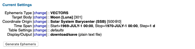
The Horizons server generates a file containing the trajectory in steps of one day for each selected object. The coordinates have a solar system barycentric origin and use as a coordinate system the ecliptic and mean equinox of reference epoch complying with the ICRF/J2000.0 reference frame.
Using the first-day position and velocities, you can then prepare the input file for the iPlanetario.awk program like the one reported in Appendix II. In this case, the location and the speeds of the planets are the one on July 1st, 1969, 16 days before the launch of Apollo 11 mission to the moon. Shall now run the program till the end of July 1969 (31 days) using an integration step of dt=1h, we can compare the percentage difference with the JPL trajectory. Figure 5 and Figure 6 show the results of the comparison.
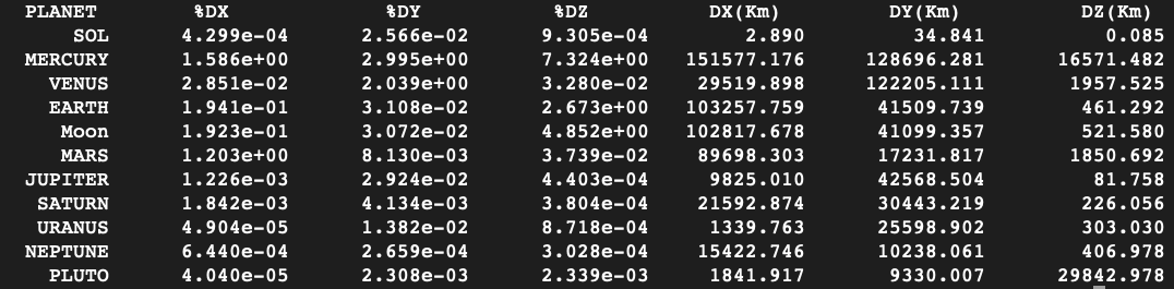
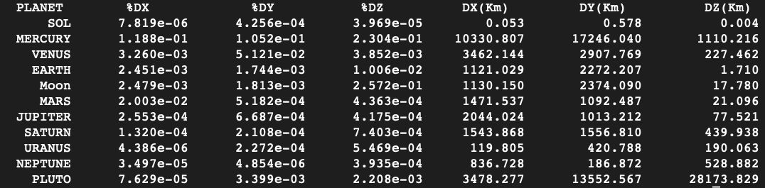
The first three columns report the average relative differences with respect to the JPL trajectories, while the last three give the average absolute differences in kilometres. By comparing Figures 5 and 6, it becomes clear that reducing the time step significantly improves the accuracy of the numerical solution. The dependence on the physical properties of the system is also evident: more massive planets are less affected by mutual perturbations, whereas lighter and faster bodies, such as Mercury, exhibit larger deviations.
Even with this relatively simple model, the predicted position of the Earth over the time span of the Apollo 11 mission differs by only a few hundred kilometres from the reference trajectory. This level of accuracy would likely be insufficient for mission-critical navigation, but it is nevertheless remarkable considering the simplicity of the approach.
At the same time, this example highlights both the power and the limitations of the earliest numerical methods. While Euler’s method provides the conceptual foundation for discretising the equations of motion, more advanced schemes—such as the Verlet or leapfrog integrators used here—are essential to achieve the level of stability and accuracy required in practical celestial mechanics. In this sense, Katherine Johnson’s intuition about relying on “old mathematics” remains deeply insightful: even the simplest ideas, when carefully extended, can lead to powerful computational tools.
BIBLIOGRAPHY
- D. Potter. Computational Physics. Wiley-Blackwell, 1973.
- Feynman, Leighton, Sands. Feynman lectures on physics. http://www.feynmanlectures.caltech.edu. Chapter 9.
- Horizons online Ephemeris System. https://ssd.jpl.nasa.gov.
If this blog was interesting and useful for you then don’t forget to press the “Like it” and “Follow it” buttons to get notification on new articles and updates!
APPENDIX I
Program in awk language to integrate the Newton equation of motion for celestial n-bodies system.
#================================================================================
#
#  NAME:  iPlanetario.awk
#
#================================================================================
# DESCRIPTION:
# This program performed a n-body simulation of a cluster of
# stars or planets. It use the leap-frog algorithm to integrate
# the Newton equation of motion.
#================================================================================
# I/O FILES :
# INPUT FILE: Read a std input file with the following format
#  LINE 1: Title
#  LINE 2: number of bodies (NB)
#  LINES 3-NB : space separated following information
#  <bodies masses>  <X> <Y> <Z> <Vx> <Vy> <Vz> <Name>
#    - masses are divided by 10^24 Kg
#    - Position in astronomical units (AU)
#    - Velocities in AU/Day
#  Example:
#  POSITION AND ORBITAL VELOCITIES OF SOLAR SYSTEM PLANETS
#  2
#  1    1.989e6      0.      0.      0.    0.     0.      0.   SOLE
#  2    0.330  -3.016E-01 -3.311E-01 -2.298E-04  1.536E-02 -1.734E-02 -2.826E-03 MERCURY
#================================================================================
#  OUTPUT FILE: The name of each body is used as filename containing the trajectory of the
#          body.
#  FILE EXAMPLE: P_MERCURY.out
#  -3.00849259e-01  -3.31952335e-01   -3.71157034e-04
#  -3.00077609e-01  -3.32815098e-01   -5.12462809e-04
#  -2.99303492e-01  -3.33675124e-01   -6.53764370e-04
#  ...
#======================================================================
# USAGE:
# gawk -f iPlanetario.awk <fname> <siml>  <dt> <sf>
# <fname>: Name of the input file
# <siml> : Lenght of the simulation in days (default = 365)
# <dt>   : time step in seconds (default dt=24*3600)
# <sf>   : Frequency of saving trajectory data (coordinated and velocities)
#          in seconds (default dt=24*3600)
#======================================================================
# Version:       1.0
# Created:       2019-07-04 20:53
# Copyright (C): 2019 Danilo Roccatano
#======================================================================
#======================================================================
#
# FUNCTIONS
#
function Calc_starting_vel() {
#
# Calculate the starting velocity at dt/2
#
    for (i=0;i<Nb;i++) {

        AX[i]=0.
        AY[i]=0.
        AZ[i]=0.
        #
        # Calculate all the forces on each planet
        #
        for (j=0;j<Nb;j++) {
            if (j!=i) {
                D2=(X[i]-X[j])^2+(Y[i]-Y[j])^2+(Z[i]-Z[j])^2
                D=sqrt(D2)
                Ac=-G*mass[j]/D2
                AX[i]=AX[i]+Ac*(X[i]-X[j])/D
                AY[i]=AY[i]+Ac*(Y[i]-Y[j])/D
                AZ[i]=AZ[i]+Ac*(Z[i]-Z[j])/D
            }
        }
        VX[i]=VX[i]+AX[i]*dt*0.5
        VY[i]=VY[i]+AY[i]*dt*0.5
        VZ[i]=VZ[i]+AZ[i]*dt*0.5
    }
}

function Read_Input_File() {
    #
    # Read input file
    #
    getline < fname
    getline < fname
    Nb=$1

    for (i=0;i<Nb;i++) {
        getline < fname
        mass[i]=$2*MU
        X[i]=$3*AU
        Y[i]=$4*AU
        Z[i]=$5*AU
        VX[i]=$6*VCV
        VY[i]=$7*VCV
        VZ[i]=$8*VCV
# read the nameof the system
        sname[i]=$9
    }
}

#==============================================================================
# MAIN
#==============================================================================
BEGIN {
#==============================================================================
# Constants
#
# AU    : Astronimical Unit
# G     : Universtal gravitation Constant
# MU    : Mass unit
# K2M   : Km to meter
# D2S   : Days to second
# VCV   : Convert velocities
# nsteps: total number of simulation step
##
    G=6.67430e-11
    AU=1.496e11 #m
    MU=1e24
    K2M=1000
    D2S = 24*3600
    VCV=AU/D2S

#################################################
# Read the command line
#################################################
#
# Name of the input file
    fname = ARGV[1]
# Lenght of the simulation in days
    ARGV[2]?siml=ARGV[2]:siml=365
# Time step in seconds
    ARGV[3]?dt=ARGV[3]:dt=D2S
# Frequency of saving coordinates and velocities
    ARGV[4]?sf=ARGV[4]:sf=D2S
    nsteps=siml*D2S/dt

#################################################
# Read input file
#################################################
    Read_Input_File()

#################################################
# WRITE THE SUMMARY OF SIMULATION PARAMETERS
#################################################
    for (i=0;i<Nb;i++) {
        print "#DATA FILE NAME          : ", fname  > "P_"sname[i]".out"
        print "#SIMULATION LENGTH (days): ", siml   > "P_"sname[i]".out"
        print "#TIME STEP (s)           : ", dt     > "P_"sname[i]".out"
        print "#NUMBER OF STEPS         : ", nsteps > "P_"sname[i]".out"
        print "#SAVING FREQUENCY (s)    : ", sf     > "P_"sname[i]".out"
    }

##################################################
# Initialize the velocities at dt/2
##################################################
    Calc_starting_vel()

##################################################
# Main Loop
##################################################
    tt=0.0
    for (t=1;t<=nsteps;t++) {
        for (i=0;i<Nb;i++) {
            # update the new position
            X[i]=X[i]+VX[i]*dt
            Y[i]=Y[i]+VY[i]*dt
            Z[i]=Z[i]+VZ[i]*dt
# clean the accelerations
            AX[i]=0
            AY[i]=0
            AZ[i]=0
            #
            # Calculate all the forces on each body
            #
            for (j=0;j<Nb;j++) {
                if (j!=i) {
                    D2=(X[i]-X[j])^2+(Y[i]-Y[j])^2+(Z[i]-Z[j])^2
                    D=sqrt(D2)
                    Ac=-G*mass[j]/D2
                    AX[i]=AX[i]+Ac*(X[i]-X[j])/D
                    AY[i]=AY[i]+Ac*(Y[i]-Y[j])/D
                    AZ[i]=AZ[i]+Ac*(Z[i]-Z[j])/D
                }
            }
            # update the new positions
            VX[i]=VX[i]+AX[i]*dt
            VY[i]=VY[i]+AY[i]*dt
            VZ[i]=VZ[i]+AZ[i]*dt
            if (tt%sf == 0) {
                printf "%15.8e  %15.8e   %15.8e  \n", X[i]/AU,Y[i]/AU,Z[i]/AU > "P_"sname[i]".out"
            }
        }
        tt+=dt
    }
}
APPENDIX II
EXAMPLE OF INPUT FILE: The starting position and velocities 9 planets of the Solar System at A.D. 1969-Jul-01 00:00:00.0000 TDB. The ephemeris have been obtained from Horizons online Ephemeris System of the Solar System Dynamics Group at the Jet Propulsion Laboratory in Pasadena (USA).
POSITION AND MEAN ORBITAL VELOCITIES OF SOLAR SYSTEM PLANETS (on 1/7/1969)
 11
   1    1.989e6     4.501422142050814E-03 8.265096431911833E-04 -6.106498754821928E-05 -3.             725998016167921E-07 5.629018018191787E-06 -1.420343330057636E-08 SOL
    2      0.330 3.626352905971110E-01 -3.112613637670733E-02 -3.556949387212367E-02    -2.936459346589251E-03  2.929519404193396E-02  2.661199336367969E-03 MERCURY
    3      4.872  6.434726285492286E-01 -3.454394151201869E-01 -4.166240919470099E-02     9.516484358480345E-03  1.770408177673933E-02 -3.091459518364233E-04 VENUS
    4      5.972  1.707701318320183E-01 -1.002143528594855E+00 -1.256995866771295E-04     1.668497591651540E-02  2.752898669289915E-03 -8.323100509758512E-08 EARTH
    5    0.642   -6.669858220909308E-02 -1.458105888577555E+00 -2.885595380269896E-02     1.450798593015611E-02  5.244375487322264E-04 -3.467167007807005E-04 MARS
    6    1898 -5.376385639107029E+00 -8.726835067297002E-01  1.240832480992071E-01     1.122255348949764E-03 -7.096896640081010E-03  4.095137444408094E-06 JUPITER
    7     568  7.884725882151399E+00  4.851428514519507E+00 -3.981641564307521E-01    -3.226967396201162E-03  4.740175258901204E-03  4.511263076949473E-05 SATURN
    8     86.8 -1.826473469434352E+01 -1.177885710585230E+00  2.326769071350472E-01     2.237727077038867E-04 -4.108566058385769E-03 -1.826199809165856E-05 URANUS
    9    102.0 -1.604710777852071E+01 -2.571063138942750E+01  8.990992317848128E-01     2.642815824514614E-03 -1.643946715455203E-03 -2.678926484808933E-05 NEPTUNE
   10      0.0146 -3.048235507172484E+01  2.734455614187439E+00  8.524022429973490E+00     3.221949947061528E-04 -3.306300878753190E-03  2.734922740068579E-04 PLUTO
   11      0.073  1.718200895379193E-01 -1.004286292375689E+00 -3.046288847913102E-04     1.726098619408255E-02  3.018131142325193E-03  2.792664511938875E-05 Moon


Pingback: Apollo Blackboard Calculation - BlackboardSub