Calculus in a Nutshell: the Definite Integral of Monovariate Functions |

The definite integral is the key tool in calculus for defining and calculating quantities important to mathematics and science, such as areas, volumes, lengths of curved paths, probabilities, and the weights of various objects, just to mention a few.

The idea behind the integral is that we can effectively compute such quantities by breaking them into small pieces and then summing the contributions from each piece.

Riemann’s definition of integral

Figure 1 show that the area under a curve 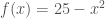$f(x)=25-x^2$ can be approximated using rectangular strips of different size as the sum (also called upper sum):

$\displaystyle { \mathcal{A} \approx S_{upper}^{p=2} = 25\sum\limits_{i=0}^{n} f(x_i)(x_{i+1}-x_i)} \ \ \ \ \ (1)$

Figure 1: Two Riemann partitions of upper sums for the function $f(x)=25-x^2$ .

Figure 1: Two Riemann partitions of upper sums for the function $f(x)=25-x^2$ .

By varing the number of strips the approximation of the integral caan be improved. In the example given in the Figure 1a there are two strips therefore the area is given by

${\mathcal{A}\approx S_{upper}^{p=5} = 25\times \frac{5}{2} + 25\times\frac{3}{4} \times \frac{5}{2} = 25\left( \frac{5}{2}+ \frac{15}{8}\right) = 25\frac{35}{8} = 109.375}$ .

In the partition in Figure 1b the interval is $\Delta x=1$ and the new sum is given by

${\mathcal{A}\approx S_{upper}^{p=5} = 25 + (25-1) + (25-4) + (25-9)+(25-16)=95 }$

We can also use the lower sums to approximate the function as shown in Figure 2.

Figure 2: Riemann partitions of lower sum with 5 partitions for the function $f(x)=25-x^2$ .

It gives us the approximate area of

${\mathcal{A}\approx S_{lower}^{p=5} =(25-1) + (25-4) + (25-9)+(25-16)=70 }$

Therefore the correct area is between the two summations

$S_{lower} < \mathcal{A} < S_{upper}$ ,

and if we increase the number of rectangles we can define the area as a limit of the value of the two summations. This limit is also very close to the one that we got using rectangles defined using the Middle Point Rule (Figure 3). In this case, the are is given by

${\mathcal{A}\approx S_{lower}^{p=5} =(25-\frac{1}{4}) + (25-\frac{9}{4}) +(25-\frac{25}{4})+(25-\frac{49}{4})+(25-\frac{81}{4})=83.75 }$

that is only 0.5 % different from the analytical value (83.33) of the integral.

Figure 3: Riemann partitions of middle point sum with 5 partitions for the function $f(x)=25-x^2$ .

Therefore, the definition of the Riemann integral require a passage to the limit of the infinitesimal partition of the area underneath the interval limits. Given the interval ${[a;b]}$ the size of the interval is given by the number ${n}$ of segments ${\Delta x=\frac{b-a}{n}}$ , the Riemann integral is defined as

$\displaystyle { \begin{array}{lll} \mathcal{A}&=&\lim_{\Delta x\rightarrow0} \sum\limits_{i=1}^{n} \!f(x_i)\Delta x\\ &=& \int_a^bf(x)dx\\ \end{array}} \ \ \ \ \ (2)$

Rigorously the Riemann integral is defined as follows

Some Definitions

Partition. Let $a<b$ be real number. A partition P of the interval $[a,b]$ is a finite subset of real numbers $x_0,\dots,x_n$ such that $a=x_0 < x_1 < \dots x_{n-1}=b$ . We write $P=x_0,x_1,\dots,x_n$ .

Norm of a Partition. We define the norm of partition P, written $||P||$ , to be largest of all the subintervall widths. If $|| P ||$ is a small number then all the subintervalls in the partitionP have a small width.

The Riemann Integral

The $f(x)$ be a function definied on a closed interval $[a,b]$ . The number $S$ is the definite integral of $f(x)$ over $[a,b]$ and that S is the limit of the Riemann sum:

$\sum_{i=1}^n f(t_i)\Delta x_j$

if the following condition is satisfied:

Given any number $\epsilon >0$ there is a corresponding number $\delta >0$ such that for every partition $P=x_0,x_1,\dots,x_n$ of $[a,b]$ with $||P||< \delta$ and any choice of $t_k$ in $|x_{k-1}-x_k|$ , we have

$\lvert \sum_{i=1}^n f(t_i) \Delta x_i-S \rvert < \epsilon$ .

Definite integral properties

Here a list of some important properties of the definite integral:

Association: ${\int_a^b \left(f(x)+g(x)\right) dx = \int_a^b f(x)dx+\int_a^b g(x)dx} \ \ \ \ \ (3)$

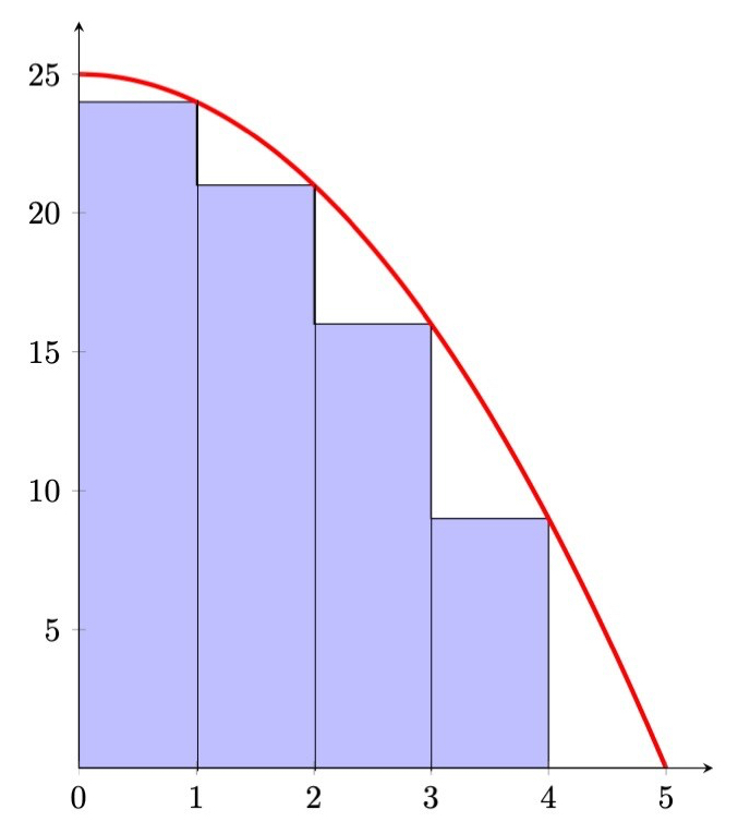
Linearity: ${\int_a^b cf(x)dx = c\int_a^b f(x)dx} \ \ \ \ \ (4)$

Partition: ${\int_a^b cf(x)dx = \int_a^c f(x)dx+\int_c^b f(x)dx } \ \ \ \ \ (5)$

Antisymmetry: ${\int_a^b cf(x)dx = -\int_b^a f(x)dx} \ \ \ \ \ (6)$

Fundamental Theorem of Calculus

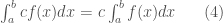
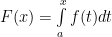
The definite integral is defined as $F(x)=\int \limits_{a}^{x}f(t)dt \ \ \ \ \ (7)$

The function F(x) gives the area under the graph of ${f(t)}$ from a to x when ${f(t)}$ is nonnegative and ${x > a}$ .

If we denote the area between ${x}$ and ${x+h}$ as ${F(x+h)-F(x)}$ then

$\displaystyle F(x+h)-F(x) \approx hf(x) \ \ \ \ \ (8)$

Theorem: If ${f}$ is continuous function on ${[a, b]}$ , then ${F(x) = \int\limits_{a}^{x}f(t)dt}$ is continuous on ${[a, b]}$ and differentiable on ${(a, b)}$ and its derivative is ${f(x)}$ :

$\displaystyle F'(x)=\frac{d}{dx}\int\limits_{a}^{x}f(t)dt=f(x) \ \ \ \ \ (9)$

Proof:

$\begin{aligned} \frac{d}{dx}\int_a^x f(s)ds &= lim_{h \rightarrow 0}\frac{\int_a^{x+h} f(s)ds-\int_a^{x} f(s)ds}{h} \\ &= lim_{h \rightarrow 0}\frac{\int_x^{x+h} f(s)ds}{h}\\ &= lim_{h \rightarrow 0}\frac{hf(s)}{h} \\ &= f(x) \end{aligned}$

$\Box$

Consider two functions ${F(x)}$ and ${G(x)=F(x)+c}$ with c a constant. Then

$\displaystyle \frac{dF(x)}{dx}=f(x)=\frac{dG(x)}{dx} \ \ \ \ \ (10)$

Thus indefinite integrals are denoted as

$\displaystyle \int f(x)dx=F(x)+c \ \ \ \ \ (11)$

Definition of Integral as antiderivative

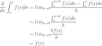
Thus in the limit that ${h \rightarrow 0}$ , we obtain

$F'(x)=\frac{dF(x)}{dx} =\lim_{h \rightarrow 0} \frac{F(x+h)-F(x)}{h} =f(x) \ \ \ \ \ (12)$

Therefore, the function of ${F(x)}$ is the inverse of the derivative (or antiderivative) of $f(x)$

$\begin{aligned} \frac{d}{dx}\int_a^b f(s)ds &= \frac{d}{dx}\int_a^b F'(s)ds \\ &= lim_{h \rightarrow 0}\sum_{n=1}^N F'(a+(n-1)h)h \\ &= lim_{h \rightarrow 0}\sum_{n=1}^N \frac{\left[F(a+nh)-F(a+(n-1)h)\right] h}{h}\\ &= lim_{h \rightarrow 0}\sum_{n=1}^N {\left[F(a+nh)-F(a+(n-1)h)\right]} \end{aligned}$

By examining the last expression it is easy to find that only the values for ${n=1}$ , ${-F(a)}$ and the one for n=N, ${F(b)}$ do not cancel out giving the demonstration of the following theorem.

Theorem: If ${f}$ is continuous at every point in ${[a, b]}$ and ${F}$ is any antiderivative of ${f}$ on ${[a, b]}$ , then $\displaystyle \int_a^bF(x)dx=\left[F(x)\right]_a^b=F(b)-F(a) \ \ \ \ \ (13)$

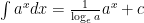
Some example indefinite integrals

${\int adx = ax+c}$
${\int x^ndx = \frac{1}{n+1}x^{n+1}+c}$ where ${n\neq-1}$
${\int\frac{1}{x}dx=lnx + c}$
${\int a^xdx=\frac{1}{\log_e{a}}a^x+c}$
${\int e^xdx=e^{x}+c}$
${\int \cos(x)dx=\sin{x}+c}$
${\int \sin(x)dx=-\cos{x}+c}$

Substitution method

$\displaystyle \frac{d f(g(x))}{dx}=f'(g(x))g'(x) \ \ \ \ \ (14)$

$\displaystyle \int f'(g(x))g'(x)dx= f(g(x))+c \ \ \ \ \ (15)$

or using the substitution ${y=g(x)}$ and ${dy=g'(x)dx}$

$\displaystyle \int f'(y)dy= f(y)+c \ \ \ \ \ (16)$

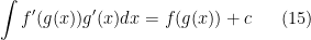
Integral by Parts Method

The derivative of a product of two functions ${(fg)'=f'g+fg'}$ , can rearrange be rearranged as ${f'g=(fg)'-fg'}$ . By taking the integral of all the terms, we can write