Molecular interactions and force fields |

At quite uncertain times and places,
The atoms left their heavenly path,
And by fortuitous embraces,
Engendered all that being hath.
And though they seem to cling together,
And form ‘associations’ here,
Yet, soon or late, they burst their tether,
And through the depths of space career.
James Clerk Maxwell

From ‘Molecular Evolution’, Nature, 8, 1873. In Lewis Campbell and William Garnett, The Life of James Clerk Maxwell (1882), 637.

Molecular forces are originated by the interactions of the electronic clouds of the atoms in the molecular systems. A full treatment of these interactions also accounting for the dynamics of the nuclei requires the solution of the time-dependent Schroedinger equation (the top of the modeling pyramid). This approach would provide a more accurate physical representation of the behavior of the systems in time. However, as pointed before, nowadays this approach is impracticable due to the enormous amount of computer resources need to accomplish this task even for relatively small peptides in water systems. The solution to this impasse is the application of the so-called lex parsimoniae or Ockham’s razor, a powerful approach in problem-solving to get rid of the redundant complexity. In this case, the law of parsimony suggests changing the level of scale and account of the hidden degree of freedom using an effective or mean field potential.

Force fields

As mentioned in the introduction of the chapter, the atomic interactions in the classical MD are treated using analytic functions. The sum of these functions, usually referred as force field function or effective potential, $V(r_1, \dots , r_N:{s})$ , depends on the atomic coordinates of the system $(r_1, \dots, r_N)$ and on number M of scalar parameters ${s}={s_1,\dots, s_M}$ defining e.g. force constants, equilibrium distances and angles, partial atomic charges, Lennard-Jones parameters. As we will see later, these parameters can be obtained from experimental data and/or from quantum mechanics calculations. The different terms composing the force field potential involve the interaction of a different number of particles. Therefore we can classify the potential as 2-bodies, three-bodies and in general as N-bodies terms. This simply means that the mathematical expressions are functions from two until N atoms coordinates, respectively.

$V({\bf{r}}, s) = \underbrace{\sum_{i, j} V^{(2)}({\bf{r}}_i, {\bf{r}}_j;s)}_\text{2 atoms inter.} + \dots + \underbrace{\sum_{all} V^{(N)} ({\bf{r}};s)}_\text{N atoms inter.}$

an example of force field, used in many programs for MD simulations, is the following:

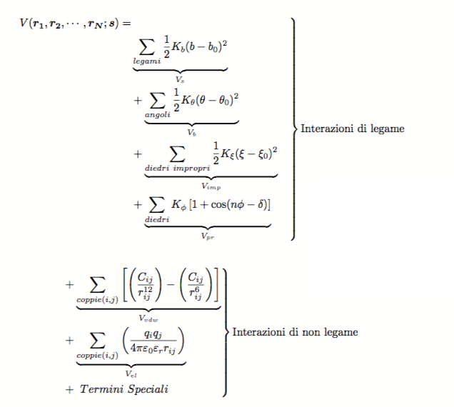
Equazione 1: an example of force field used in MD simulations.

Bonded interactions

The bonded interactions are usually described using functions depending on the coordinates of 2 to 4 particles. These interactions generally describe harmonic motions with force constants obtained from experimental crystallographic and spectroscopic data.

Bond vibrations

The first term ( $V_{\beta}$ ) in the force field equation represents the energy of bond vibration. It is usually represented as a harmonic term where $b_0$ represents the equilibrium bond length and $K_b$ the force constant, which changes according to the bond type. In some force fields, the Morse function is used:

$V_M(b)=\sum_{legami} D_e \left\{e^{[ - k_b(b-b_0) ]} -1 \right\}^2$

where the parameter $D_e$ represents the energy of bond dissociation and $k_b = \omega \sqrt{\mu/2D_e}$ , where $\omega$ is the vibration frequency and $\mu$ the reduced mass, the force constant. This type of interaction is used to provide a more accurate description of large displacements of the bond distance b and a higher accuracy in the reproduction of the infrared vibrational spectra of molecular systems. It can also be used to simulate bond breaking processes.

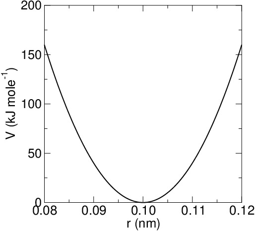
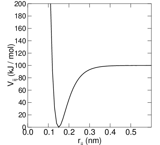
Figura 1: Examples of bond vibration potential: harmonic type (on the left); Morse type (on the right).

Bond angle vibration

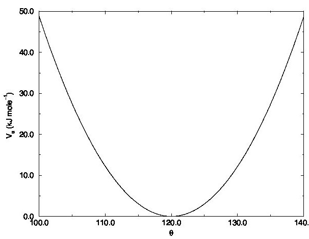
The second term in force field Equation describes the interaction energy due to the deformation of the bond angle. This is a three-bodies interaction term since it depends on three atoms. The function represents harmonic angular vibrations, where $\theta_0$ is the reference value of the bond angle and $K_{\theta}$ the force constant. The bond angle interaction term can have different functional forms.

f_angle

Figure 2: Example of bond angle vibration harmonic potential.

In some force fields, mixed bond-angle terms of type $K_{b\theta}[b-b_0][\theta-\theta_0]$ are used to account for the coupling variations of the bond length and bond angles. In more complex expressions also the dihedral angles are taken into account for this mixing.

Four body interactions

In the Equ. 1, two terms are used to describe the following four-bodies interactions.

Improper dihedral vibrations

The first one describes the so-called improper dihedral angle vibrations. This term is used in order to account for the deformation of tetrahedral and planar geometries. The need to maintain tetrahedral geometries is due to the fact that in some force fields, apolar aliphatic hydrogens are not considered explicitly, but their effect is included by modifying the interaction functions of the atoms to which they are bound. In this way, chiral aliphatic carbons have only three coordinating atoms, this involves that during the simulation it can happen that these invert their chirality. Using improper dihedrals, this effect can be avoided by introducing an extra potential that keeps in place the right stereochemistry. The improper dihedral angle, i-j-k-l, is defined as the angle between the plane that is spanned by atoms i, j, and k and the plan spanned by atoms j, k, and l.

impr_def

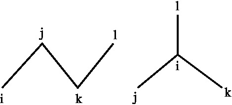
Figure 3: Definitions of improper dihedrals.

Torsion potentials

The other term for the four atom interactions describes the energy involved in the rotation around bonds. It is usually described as a sinusoidal function where $K_\phi$ is the force constant, n the number of minima and $\delta$ the phase.

f_dih

Figure 4: Example of torsion potential.

Derivation of the bond interaction parameters

In order to determine the parameters for the force fields, two paths are usually followed.
The most elegant method is to optimize these parameters by fitting to an energy function derived from quantum-mechanical calculations on small molecules. Bond and bond-angle can be obtained by normal mode analysis, while the dihedral term can be acquired by conformational analysis of the molecule around the specific bond. Alternatively, it is possible to optimize the force field parameters using experimental data: crystallographic structures, infrared and NMR spectroscopy, dynamic and thermodynamic properties of liquids as density and enthalpy of vaporization, free energy of solvation, just to mention some [Jorgensen83, Lifson83, Giglio69]. Using this approach, the model obtained is able to reproduce the experimental macroscopic properties of bulk liquids.

Non-bonded interactions

The last terms in Equ.~\ref{equ:forcef} describe the interactions between non-bonded atoms. The two terms are usually modeled using pair interaction functions describing van der Waals and Coulombic interactions of the atom pairs i and j having partial charges $q_i$ and $q_j$ at distance $r_{ij}$ .

Van der Waals interactions

The short-range interactions are usually described using Lennard-Jones functions. The Lennard-Jones potential is composed of two terms that describe a repulsive and an attractive type interaction:

$\displaystyle V_{LJ} (r) = \underbrace{\frac{C^{12}}{r^{12}}}_{Termine~repulsivo} - \underbrace{\frac{C^6}{r^6}}_{Termine~attrattivo} \ \ \ \ \ (4)$

$C^{12}$ and $C^6$ are constants that can be obtained from experimental data or from quantum mechanical calculations. The short range repulsion term can have different functional forms. In the case of the Buckingham [Buckingham38] potential, the exponential term $b\exp [ – ar]$, with $a$ and $b$ being two constants, is used. The exponential term provides a better description of the potential at the short range since it is less steep than the LJ one. In the case of liquid state simulation, it provides a more accurate description of the first peak in the pair distribution function.

$\displaystyle C^6_{ij} = \frac{3}{2} \frac{\alpha_i \alpha_j}{\sqrt{\frac{\alpha_j}{N_j}} + \sqrt{\frac{\alpha_i}{N_i}}} = \frac{\alpha_i \alpha_j}{{\alpha_j}^2{C_{jj}^6} + {\alpha_i}^2{C_{ii}^6}} \ \ \ \ \ (5)$

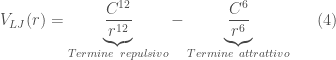
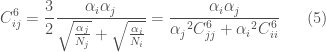
The attractive term in Equ.~\ref{lennardjones} describes the contribution of the non-bonded interactions of the so-called dispersive or London forces [London30, Israelachvili85]. The values of the constants $C^6_{ii}$ (homotype interactions) can be obtained from the atomic polarizability of the ith atom using different equations like
the equation of Slater-Kirkwood [Margenau69]:

in which N represents the effective atomic electron number and $\alpha$ the polarizability, $N_i = 16{(C_{jj}^6)}^2/9\alpha_i^3$ . The values of $C^{12}_{ij}$ can be obtained from experimental measurements of the virial coefficient (see Box\ref{BoxVir}) or from crystallographic and thermodynamic data.

NOTE: The equation of state for a real gas can be expressed using the Virial formula

$\frac{PV}{nRT} = 1 + \frac{B}{V} + \frac {C}{V^2} + \cdots$

where $B$ and $C$ are the second and third coefficients of the Virial, respectively. For a good description of a gas in ideal conditions (very low dilution) it is already sufficient to consider only the $B$ coefficient. Applying the kinetic theory of gases, Rayleigh has found an analytic expression that connects $B$ to the atomic interaction function:

$B = 2\pi N\int_0^{infty} \left(1-\exp{-\frac{V(r)}{RT}}\right)r^2 dr$

where r is the distance between the interacting molecule and the reference one. By replacing in V(r) the expression of the Lennard-Jones equation, it is possible to obtain an expression that allows determining the parameters $C_{jj}^6$ and $C_{jj}^12$ , by measuring $B$ at different temperatures. Indeed the procedure is more complex since it is not possible to obtain unique solutions from the previous expression. Therefore, to reduce this indetermination, the parameter $C_{jj}^12$ is determined, while the parameter $C_{jj}^6$ is estimated from the Slater-Kirkwood equation.

In the original form of the Lennard-Jones equation, the $C^{12}$ and $C^6$ are expressed in terms of $\sigma$ and $\epsilon$ values that represent the distance at which the function has zero value and the value of the function is at its energy minimum (that is located at $r_{min}={2}^{1/6}\sigma)$ .

$V_{LJ} = 4 \epsilon \left[\left(\frac{\sigma}{r}\right)^{12} - \left(\frac{\sigma}{r}\right)^{6}\right]$

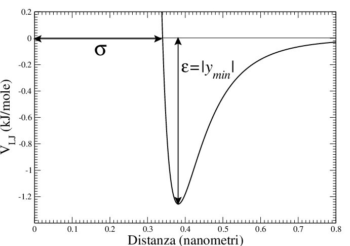
The values of $\sigma$ and $\epsilon$ are related to the two types of interacting atoms, they can be arranged in order to obtain the corresponding LJ parameters.

LJcurves

Figure 5: Example of Lennard-Jones potential.

Various types of combination rules exist, in one of the most widely used the new parameters are obtained in the following way:

$\displaystyle \sigma_{ij} = \frac{\sigma_{ii}+ \sigma_{jj}}{2} \ \ \ \ \ (9)$

$\displaystyle \epsilon_{ij} = \sqrt{\epsilon_{ii}\epsilon_{jj}} \ \ \ \ \ (10)$

The interactions between atoms covalently bound or not separate from each other by more than two bonds normally are not calculated. On the contrary, in the case of interactions between atoms separated by three bonds, the parameters of the LJ functions are properly reduced in order to avoid strong repulsions caused by the distances being too short. The parameters $C^{12}_{ij}$ for the united atoms (CH-, $CH_{2}-, CH_{3}-$ ) are estimated to correctly reproduce the crystal density of small molecules at constant pressure.

Electrostatic interactions

The electrostatic interactions are generally described using a coulomb term. Every atom of the system is provided with a partial atomic charge calculated using a quantum-mechanical method. The choice of the relative dielectric constant, $\varepsilon_r$, is still a matter of discussion in case one wants to simulate non-homogenous molecular systems, as proteins in water. Different values have been used that vary from $\varepsilon_r=1$ to $\varepsilon_r=8$ , or complex functions proportional to the distance $r_{ij}$ [McCammon77, Brooks83, Weiner86]. These approximations physically only show poor realistic behavior, the better solution to this problem would be the inclusion of the atomic polarizability that would allow obtaining the correct electric field in every point of the simulated system. In order to include the polarizability it is necessary to introduce a more complex electric field equation that accounts for the presence of induced electric dipoles on the single atoms:

$\Delta {\bf{p_i}} = \alpha_i{\bf{E_i}} = \alpha_i \sum_i^N \sum_{j \neq i}^N {\bf{T_{ij}}} \left( {\bf{p_j}} + \Delta {\bf{p_i}} \right)$

where N is the atom number of the system, ${\bf{p_i}}$ and $\delta {\bf{p_i}}$
are the dipole moment and the induced dipole moment on the ith atom, respectively. Finally, the polarizability tensor is defined as follow:
${\bf{T_{ij}}} = \frac{1}{4\pi\epsilon_0 {\bf{r}}^3}\left( \frac{3{\bf{r_i}}{\bf{r_j}}}{{\bf{r_ij}}^2} -1\right)$

The previous equations set a system of 3N equations of 3N unknowns (each for the x, y, z components of every atom) that can be numerically solved. Another different way to introduce the polarizability in the simulated system is the use of the dummy charged particle, localized on each atom and bonded together using harmonic springs with an opportune force constant (Drude’s harmonic oscillators). The deformation of the spring resulting from the interactions with other atoms, produce a charge separation of the atoms and produce an induced dipole.

The hydrogen bond

Another important molecular interaction is the hydrogen bond. The term \em hydrogen bond \em is used in order to indicate all those atomic contacts in which the internuclear distances, $R_{H-X}$ and $R_{H-Y}$ between a hydrogen atom (H) and two other atoms X and Y, are meaningfully smaller than the sum of their van der Waals radii(r): ( $R_{H-X}<r_H^{vw}+r_X^{vw}$ , e $R_{H-Y}<r_H^{vw}+r_Y^{vw}$ ). The hydrogen bond, differently from the normal dispersion interaction (London forces), has stronger interaction and a geometric dependence [Lippert76]. The nature of this interaction is mainly electrostatic, for this reason, in most of the force field, this interaction is modeled by using appropriate values for LJ and partial charges on the atoms involved in the binding [Lifson79, Jorgensen88, Hagler89, Hermans84]. In other force fields, the HB is modeled using special interaction functions as [Levitt83, Brooks83, Weiner86]:

$V(r) = \frac{A}{r^{12}} - \frac{C}{r^{10}}$

usually multiplied by a function of the angular orientation of the atoms involved.

Special interaction potentials

It is possible to add special terms to the force field potential function that describe the effect of external forces, that restrain the dynamics of the systems. In the case of proteins
or nucleic acids, these restraints confine the conformational space accessible to the molecule based experimental data. When these data are from X-ray diffraction or NMR, or other structural spectroscopic techniques, these potential restraints allow refining the molecular structure. Two examples of these potentials are reported in the following paragraphs.

Positional restraints

In case you want to keep a set of atoms vibrating around fixed positions in space, then
it is possible to define a harmonic potential that restraints the atoms to vibrate around a reference position $r_{i}^{ref}$ :

$V({\bf{r}})=\frac{1}{2} \sum_{N}\left(r_{i}-r_{i}^{ref}\right)^2$

This potential restraint is useful for simulations of solid surfaces, or to avoid structural deformation of large macromolecules during the equilibration of the surrounding solvent.

Restraint potential based on the crystallographic structure factors

The x-ray diffraction measurements provided the so-called structure factors, $F(hkl)$ , and if the data are very accurate and redundant the phase factors, $\alpha(hkl)$ , that describe the electron density around the atoms of the crystallographic structure. The value of the amplitude can be used to define the following restraint potential:

$V_{X}= \frac{1}{2}K_{X} \sum_{hkl}\left[F_{calc}(hkl)-F_{obs}(hkl)\right]^2$

where $F_{calc}(hkl)$ are the amplitudes of the structure factors calculated from the MD simulation [Brunger87, Brunger91]. The values of the force constants are usually varied during the refinement procedure. Large values improve the agreement with the experimental data but if the values become too large, the flexibility of the molecule can be strongly reduced \cite{vanGunsteren84} compromising the efficiency of the refinement procedure. The use of the average quantities make the potential not conservative (cause of the time dependence) and, therefore, it renders necessary to dissipate the generated heat by coupling the system to an external thermal bath [Torda90].

Distance dependent restraint potentials

The NMR spectroscopy provides accurate data on the average inter-protonic distance (Overhauser effect), on the dihedral angles (J coupling constants) and on the chemical shift that can be used to add precious structural information to the dynamical behavior of a macromolecule in an MD simulation. In this way, it is possible to obtain molecular structures that fulfill the experimental requirements. The NOE (Nuclear Overhauser Effect) intensities from NMR experiments can be converted in a set of superior limit distances ${{\bf{r}}_{ij}^{ub}}$ between the protons i e j. This information can be included in the force field using the expression [Kaptein85]:

$V({\bf{r}})=\frac{1}{2} \sum_{NOE}\left[max(0,<r_{ij}^{-1/3}>-r_{ij}^{ub})\right]^2$

where the function MAX provide the max value between the two arguments. The values of the coupling constant $J$ can be included in the force field using the relation [Torda93]:
$V_{J}({\bf{r}})= \frac {1}{2} K_{J} \sum_{\phi_i} \left[ <J(\phi_i({\bf{r}})> - J_i^{spe}\right]^2$

The coupling constant J depends on the torsion angle $\phi_i$ between the atoms involved in the chemical shift coupling.

Finally, the chemical shifts $\sigma$ calculated from the simulation can be constrained to the experimental values $\sigma^{spe}$ using the potential function [Harvey93]:

$V_{\sigma}({\bf{r}})= \frac {1}{2} K_{\sigma} \sum_{i} \left[ <\sigma_i({\bf{r}})> - \sigma_i^{spe}\right]^2$

where the sum is calculated over all the constrained atoms. The average $< \ldots >$ in all the previous relations is calculated over the whole trajectory.

Optimization of the molecular geometry

The potential function, described in the previous paragraphs, is used in molecular mechanics to explore the conformational energy surface of small molecules. This exploration would allow searching for those conformations that are energetically localized in minimum points. An exhaustive search procedure is difficult to perform for molecules having many dihedrals. However, for the optimization of the structure to the closest minimum, it is important to eliminate possible contacts in the starting conformation of the MD simulations. In fact, incorrect molecular conformation can create problems in the integration algorithms of the equation of motion.

A molecular configuration is in a conformational energy minimum if the following condition is verified:

$\sum_{i=1}^N \frac{\partial V_{i}}{\partial \bf{r_{i}}} = 0$

where N is the total number of atoms of the system, $V_i$ is the value o the potential of the ith atom and $r_i$ the position. For large N it is too complex to find an analytical solution for the function V [[of its roots (minimum)]], therefore it is necessary to resort to numerical methods.

Among the methods used to search for local minima the most widely used are:

The steepest descent method
The conjugate gradient method

In the first case, given a molecular geometry, defined by the coordinates $\bf{r}$ , the gradient of the energy $\bf{f} = \nabla V_i$ that defines the directions along which the interaction energy is changing most rapidly, is calculated. The search for new, optimized coordinates consists of moving the components of the coordinates of each atom, by a step $\lambda$ along the vector $\bf{r} - \lambda \bf{f}$ until a minimum of V along this direction is encountered. Starting from this new geometry, $\bf{r_2}$ , the gradient is calculated again, $\bf{f_2}$ at the new position and the coordinates are moved again along this gradient towards the minimum. This procedure is repeated until the value of the gradient does not change further (the minimum of energy is reached). The method is very fast but becomes inefficient in the proximity to the minimum. The method of conjugate gradients starts in a similar fashion as the steepest descent method, but after having reached the minimum $\bf{r_2}$ along the direction $\bf{s_1} = \bf{r_2} - \lambda \bf{f}$ , it proceeds its search in the direction $\bf{s_2} = -\bf{f_2} - \beta \bf{s_1}$ where $\beta = \frac{|\bf{f_2}|^2}{|\bf{f_1}|^2}$ . In this way the direction of search, in the point $\bf{r_k}$ , is no longer the gradient of $\bf{f_k}$ but a linear combination of the new gradient and the one obtained from the previous search direction:

$\bf{s_k} = -\bf{f_k} + \beta \bf{s{k-1}}$

with $\beta = \frac{|\bf{f_k}|^2}{|\bf{f_{k-1}}|^2}$ . Therefore, this method, on the contrary to the \em steepest descent\em method, takes into account the minimization path and this allows to reduce the minimization step in the proximity of a local minimum.

One thought on “Molecular interactions and force fields”

Pingback: Calculus in a Nutshell: functions and derivatives | Danilo Roccatano

M	T	W	T	F	S	S
1	2	3	4	5	6	7
8	9	10	11	12	13	14
15	16	17	18	19	20	21
22	23	24	25	26	27	28
29	30	31

"… I seem […] only like a boy playing on the sea-shore, and diverting myself in now and then finding a smoother pebble or a prettier shell than ordinary, whilst the great ocean of truth lay all undiscovered before me". – Isaac Newton.

Molecular interactions and force fields

Force fields