Chimica Fisica: Il metodo di Hückel (Parte I)

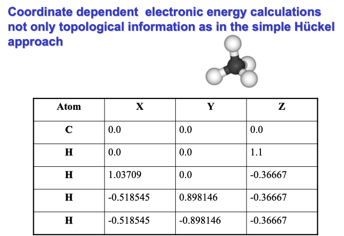
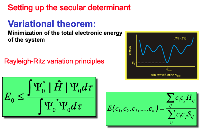
Il metodo degli orbitali molecolari di Hückel è un metodo quanto meccanico semi-empirico usato per calcolare le proprietà degli orbitali molecolari degli elettroni π in sistemi d’idrocarburici coniugati, come, per esempio, l’etilene, il benzene o il butadiene. In questa serie di articoli, ho riassunto gli aspetti principali della teoria con esempi pratici di applicazioni e programmazione del metodo.

Continue reading

Easter 2022: Modelling and Designing of Birds Eggs for 3D Printing

A box without hinges, key, or lid,
Yet golden treasure inside is hid.

JRR Tolkien, The Hobbit

Easter 2022 is at the door and the occasion for the traditional appointment to talk about eggs and their mathematical shapes. This year with the help of my sons, we have created the following Instructable for STEM education:

https://www.instructables.com/Modelling-and-Designing-of-Bird-Eggs-for-3D-Printi/

The project aims to show how to use a simple mathematical model to generate the 3D form of real bird eggs utilizing several parameters. The 3D egg models can be saved as an STL file and then printed using a 3D printer. The printed egg can be painted or modified with a CAD program to add functionalities for egg-based gadgets or toys. An example of a modification to create a LED decorated egg is explained in detail.

More recently for fun, I have published another one using the same approach:

https://www.instructables.com/The-Eggyrint/

The egg modelling topic has been covered in previous article, and the interested reader can complement the information in the Instructable with other information provided in the following articles:

https://wordpress.com/post/daniloroccatano.blog/3792

https://wordpress.com/post/daniloroccatano.blog/5171

https://wordpress.com/post/daniloroccatano.blog/6760

The Instructable gives the possibility to 3D print and modifies the 3D shape of bird eggs. It can be used for research, teaching and fun. I hope you will enjoy it, and constructive comments and suggestions are always welcome!

AUGURO A TUTTI I LETTORI UNA BUONA PASQUA E PACE IN TERRA

WÜNSCHT ALLEN LESERN FROHE OSTERN UND FRIEDEN AUF ERDEN

I WISH TO READER A HAPPY EASTER AND PEACE ON EARTH

Come Creare Modelli Tridimensionali di Conchiglie e altri Molluschi

Questo articolo è la traduzione di un recente instructable in lingua inglese sul sito Instructables teachers (https://www.instructables.com/How-to-Generate-and-3D-Print-Seashells-and-Other-M). Sull’argomento ho già scritto un altro breve articolo (anche questo in lingua inglese) nel passato, tuttavia, visto il considerable interesse ricevuto dall’instructable ( che ha vinto anche un premio runner-up nella competizione “made with math”) ho deciso di farne una traduzione per i lettori italiani del mio blog.

Continue reading

Exploring the Lotus Effect using Candle Soot

I recently published an new Instructable that is the results of some home experiments that I did some time ago (see also my previous article).

https://www.instructables.com/EXPLORING-THE-LOTUS-EFFECT-USING-CANDLE-SOOT/

It shows how to prepare these simple surfaces and make some interesting observations with them. Like the previous two Instructables, my family help me a lot in preparing it in the very short time of one day. So a big thank you to my wife, Francesco, and, in particular, to Leonardo.

Hydrophobic and super-hydrophobic surfaces are ubiquitous in the natural world. You do not need to search much to find good examples: just walk out in your garden after a light rain and look at the plenty of weed leaves pearly decorated by water droplets. If you have an ornamental pond, you may have even the chance to see floating better examples of plants having a super-hydrophobic surface. Notably, wettability in Nature is present in a different form that subtle differences in the function and effect on the water droplets. Plant leaves need to keep their surfaces clean for light-harvesting efficiency. A water repellent leaves let water drops roll over its surface and mechanically remove dust particles. This effect was first noted on leaves of the Lotus plant, and for that reason, it is also called the Lotus effect.

Several novel technological materials exploit the properties of super-hydrophobic. For example, in your kitchen, Teflon pans are used to avoid sticking food residuals and therefore easily cleaned. Your car windows are teated to let the water easily roll over the surface. 

Candle soot is an artificial material that is easy to produce and can be used to demonstrate some of the properties of the (super)-hydrophobic surface existing in nature.

The Mighty Roto-Microscope

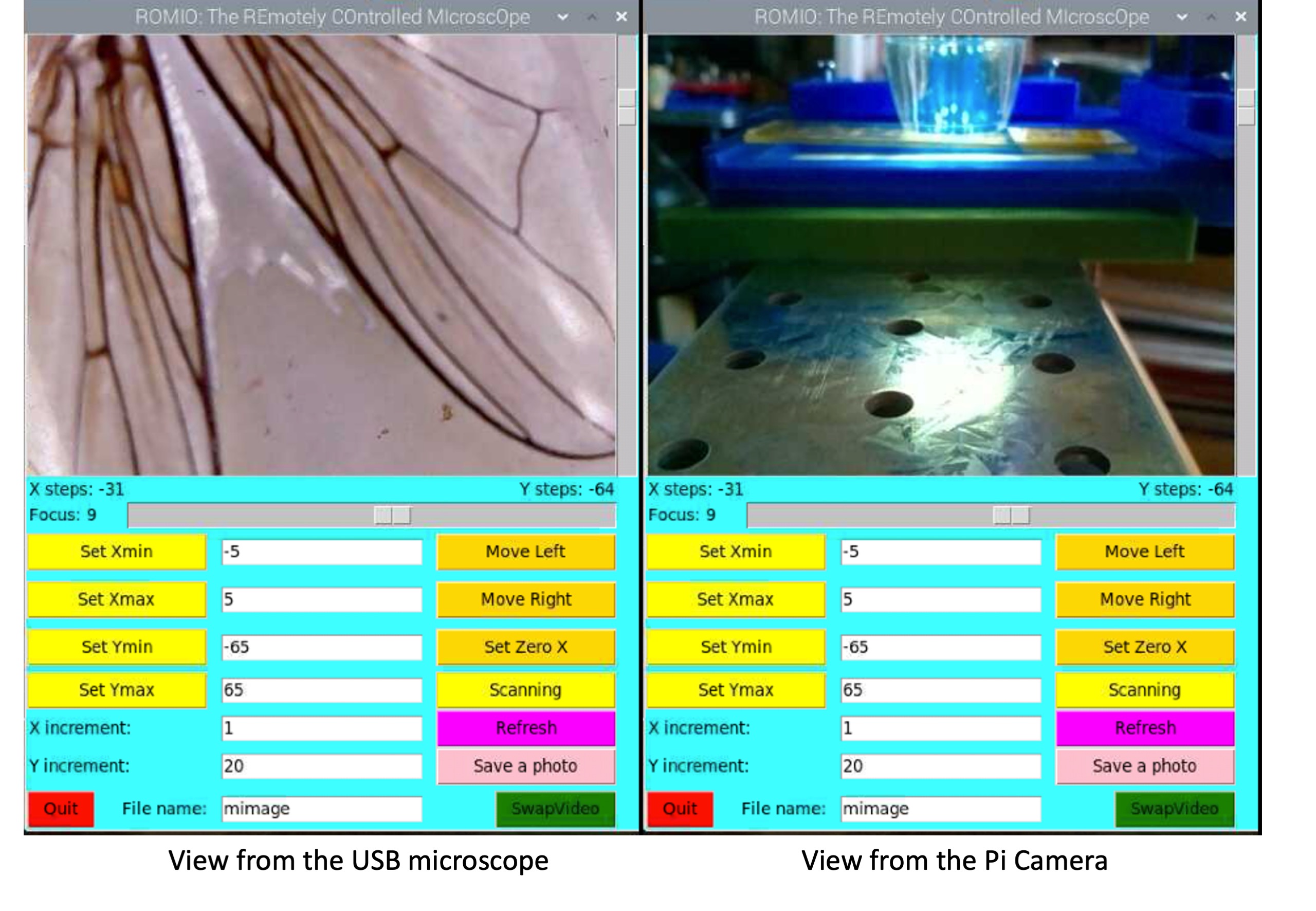
I am happy to announce our second Instructable project. Like the first one, it was a long-standing idea that was rolling in my mind for a long time. The current limited travelling mobility due to the COVID offered more time to develop this idea during my vacation. In a joyful collaboration with my son Leonardo, we managed to realize this useful device in a very short time.

This project aimed to develop a device that integrated with a cheap USB microscope allows taking 3D pictures of small samples. The project is meant to be an education STEM activity to learn using Arduino, 3D image reconstruction, and 3D printing by creating a useful piece of equipment for doing some exciting science activity. Like my previous project, it is also a moment to share good and educative time with my family and in particular, my elder son Leonardo that helped me in creating this instructable and evaluating the device as an enthusiastic STEM student. This time, also my lovely wife helps me to make a video of the assembly of the equipment!

The roto-microscope allows controlling the position of a simple USB microscope around the sample. This allows to take accurate pictures from different angles and not just from the top as in the traditional microscopes. This is not a new idea as there are professional microscopes. However, this device means to be affordable for a student and still provides some similar results and a lot of fun in building it. Other similar and excellent OpenSource projects are available (see, for example, the Ladybug microscope, the Lego microscope, and the OpenScan project), our project adds an additional option and I hope that you enjoy making it as we did!

If you find it an interesting device then instructions on how to build it are on our Instructable.

Seminar Series: Molecular Dynamics Simulation of Biomolecules

In this new series, I will post slides of seminars or lessons that I have delivered in the past years. Some of the reported information is updated, but still helpful. In some cases, I have added descriptions of the slide contents or references to other articles or the original paper where I describe my research results.
I hope you like the presentation, and remember to add your feedback and subscribe to have email notifications about my new blog posts.

In 1648, Isaac Newton published his first edition of the Principia Mathematica, one of the greatest scientific masterpieces of all time. On page 12 of this magnum opus, the famous three laws that bear his name and from which classical mathematical physics evolved are enunciated. More than 350 years after that publication, the same laws formulated to explain the motion of stars and planets remain valuable for us when trying to simplify the description of the atomic world. In the first decades of the last century, the birth of quantum mechanics marked the beginning of the detailed description of atomic physics. The equation of Schrödinger, to the same extent as Newton’s equations, allowed for the mathematically elegant formulation of the shining theoretical intuitions and the experimental data accumulated in the previous decades. Although this equation could be used in principle to describe any molecular system’s physicochemical behaviour, it is impossible to resolve analytically when the number of electrons is more than two. The invention of electronic computers after World War II facilitated the numerical solution of this equation for polyatomic systems. However, despite the continuous and rapid development of computer performance, the ab-initio quantum-mechanical approach to describe static and dynamic properties of molecules containing hundreds or even thousands of atoms, as for biological macromolecules, is still far from becoming a standard computational tool. This approach requires many calculations that can be proportional to N^{3-5}, where N is the total number of electrons in the system. It was clear that a reduction, using ad hoc approximations, of the description of the dynamic behaviour of atoms using a classic physics model would be necessary to overcome this problem. In the classical representation, the electrons on the atoms are not explicitly considered, but their mean-field effect is taken into account. Alder and Wainwright performed the first simulation of an atomic fluid using this approximation approximately 63 years ago (1957). They developed and used the method to study simple fluids by means of a model representing atoms as discs and rigid spheres. These first pioneer studies mark the birth of the classical molecular dynamics (MD) simulation technique. The successive use of more realistic interaction potentials has allowed obtaining simulations comparable to experimental data, showing that MD can be a valuable tool for surveying the microscopical properties of physical systems. The first simulations of this type were carried out by Rahman and Verlet (1964): in these simulations, a Lennard-Jones-type potential was used to describe the atomic interactions of argon in the liquid state. Another significant hallmark in this field was the simulation of the first protein (the bovine pancreatic trypsin inhibitor) by McCammon and Karplus in 1977. In the following years, the success obtained in reproducing structural properties of proteins and other macromolecules led to a great spread of the MD within structural biology studies. The continuous increase of computer power and improvement of programming languages has concurred with further refinement of the technique. Its application was progressively expanded to more complex biological systems comprising large protein complexes in a membrane environment. In this way, MD is becoming a powerful and flexible tool with applications in disparate fields, from structural biology to material science.

Continue reading

1971-2021: The Molecular Dynamics of Liquid Water turns Fifty

This year signs a landmark in the history of the molecular dynamics (MD) simulation method. Half a century ago 1971, Aneesur Rhaman and Frank H. Stillinger [1] published a pioneering work on the MD simulation of liquid water in the Journal of Chemical Physics. The journal received the article on May the 6th, 1971, and accepted it in October. Just seven years before (1964), the physicist A. Rahman (24 August 1927 – 6 June 1987) pioneered the computational method of MD when he published the first MD simulation study of liquid Argon [2]. The 1971 article is also the first MD study of a molecule in a condensed phase. It signed an important milestones water models are the most studied and used molecular models in MD simulations.

However, despite its structural simplicity, after 50 years of intense study, a perfect model for MD simulation is not yet available. By a perfect model, I mean one capable of computationally conveniently reproducing all the properties of water molecules in the range of possible applications. A water model needs to balance its computational simplicity required to keep computational costs for the simulations of large macromolecules in solution limited, and the accuracy to reproduce the physical chemistry properties accurately. For the most used but still 40-year-old models, this compromise was the equivalent of the inconveniently short blanket: pulling on one side would fit some properties but leave others loose. However, the continuous availability of inexpensive computer power and the advancements in simulation algorithms have allowed for significant progress in developing more accurate and efficient water models. In fact, several excellent models have been proposed since the R&S publication that can reproduce very well properties at 298 K or in a limited range of temperatures. In an updated but comprehensive article written 30 years later in the R&S paper, Guillot reported more than 100 proposed classic models for MD or Monte Carlo simulations published up to then [3]. Nineteen years after the publication of Guillot’s review, new and more sophisticated models have been proposed; nevertheless, the most used ones continue to bring the legacy of the R&S model.

In the late 1970s and early 1980s, the first molecular dynamics simulations of water were conducted using simplified models. These models represented water molecules as spheres interacting via pairwise Lennard-Jones potentials, capturing the intermolecular forces between the molecules. These developments in modeling water from molecular dynamics simulations have contributed significantly to our understanding of water’s structure, thermodynamics, and dynamics at the molecular level. They have provided insights into a wide range of phenomena, including solvation, hydrophobic interactions, phase transitions, and biomolecular interactions involving water molecules. In the following list, there is a summary of commonly used models for simulating water in molecular dynamics simulations.

  1. The SPC (Simple Point Charge) and SPC/E (Extended) developed by Prof. HJC Berendsen and collaborators a the University of Groningen (The Netherlands) [4] are widely used water models in molecular dynamics simulations. These models consider three atoms per water molecule but have different parameters for the Lennard-Jones potential and partial charges. The SPC/E model, in particular, has successfully reproduced various water properties, including the density and structure of liquid water.
    • Lennard-Jones Potential: The SPC models also utilize the Lennard-Jones potential to describe the van der Waals interactions between water molecules. The parameters are adjusted to reproduce various properties of water, including the radial distribution function.
    • Charges: The SPC models assign partial charges to the oxygen and hydrogen atoms in a manner that reproduces the dipole moment and electric field properties of water. These charges are carefully chosen to ensure an accurate representation of the water molecule.
  2. The TIP3P (Transferable Intermolecular Potential 3 Points) model developed by Prof. W. Jorgensen and collaborators at Yale University (USA) [4] is another widely-used water model. As the SPC model, it represents water molecules as three atoms: two hydrogen atoms and one oxygen atom. The oxygen atom has a partial negative charge, while each hydrogen atom has a partial positive charge. The model also includes harmonic bond stretching and angle bending terms to describe the covalent bonds and bond angles within water molecules.
    • Bond Stretching: The TIP3P model assumes harmonic bond stretching between oxygen and hydrogen atoms. The equilibrium bond length is typically set to 0.9572 Å, and the force constant represents the stiffness of the bond.
    • Angle Bending: The TIP3P model employs harmonic angle bending terms to describe the HOH angle. The equilibrium angle is typically set to 104.52 degrees, corresponding to the tetrahedral geometry of water.
    • Lennard-Jones Potential: The model uses the Lennard-Jones potential to describe the van der Waals interactions between water molecules. The parameters for the potential are chosen to reproduce the experimentally observed properties of water, such as the density and vaporization enthalpy.
    • Charges: The oxygen atom in the TIP3P model carries a partial negative charge, while each hydrogen atom has a partial positive charge. The charges are usually chosen to reproduce the dipole moment and electric field properties of water.
  3. The TIP4P model extends the TIP3P model by explicitly including a virtual site, referred to as the “dummy” or “massless” site, in addition to the three atoms. This dummy site is located along the HOH angle bisector and represents the lone pair of electrons on the oxygen atom. The TIP4P model improves the description of water properties, particularly the hydrogen bonding behavior.
    • Dummy Sites: The TIP4P model introduces a virtual site, referred to as the dummy or massless site, to represent the lone pair of electrons on the oxygen atom. This allows for a more accurate representation of the hydrogen bonding behavior in water.
    • Electrostatics: The TIP4P model includes a positive charge located on the dummy site, which balances the negative charge on the oxygen atom. This ensures that the model reproduces the correct dipole moment of water.
  4. Flexible Models: While rigid water models, such as TIP3P and SPC/E, assume fixed bond lengths and bond angles, flexible models introduce additional degrees of freedom by allowing parameter variations. Flexible water models, such as TIP5P and TIP4P/2005, consider the anharmonicity of bond stretching and angle bending, providing a more accurate description of water’s vibrational behavior.
    • Anharmonicity: Flexible water models, such as TIP4P/2005 and TIP5P, introduce anharmonic terms to account for the deviations from the harmonic behavior of bond stretching and angle bending. This allows for a more accurate representation of water’s vibrational properties.
    • Improved Parameters: Flexible models often incorporate refined parameters to better reproduce experimental data, such as vibrational spectra and thermodynamic properties, beyond what can be achieved with rigid models.
  5. Polarizable Models: Classical force fields typically assume fixed atomic charges on water molecules. However, water is a polar molecule whose charge distribution changes in response to its local environment. Polarizable models have been developed to capture the dynamic nature of water’s charge distribution. Polarizable force fields, such as the AMOEBA (Atomic Multipole Optimized Energetics for Biomolecular Simulation) force field, allow the partial charges on water molecules to vary with the atomic positions and local electric fields.
    • Drude Oscillators: Polarizable models, such as the AMOEBA force field, employ Drude oscillators to represent the fluctuating charge distributions in water. A Drude oscillator consists of a heavy atom (representing the oxygen atom) and a lighter particle (representing the hydrogen atom) connected by a harmonic bond.
    • Atomic Multipole Moments: Polarizable models use atomic multipole moments, including dipoles, quadrupoles, and higher-order moments, to describe the charge distribution of water molecules. The moments are allowed to vary with the positions of the atoms, capturing the dynamic nature of water’s charge distribution.

These model are the most communely used water models used in molecular dynamics simulations an din particular in simulation of biomolecular systems. The choice of model depends on the research question and the desired level of accuracy required for the simulation.

REFERENCES

  1. Rahman, A. and Stillinger, F.H., 1971. Molecular dynamics study of liquid water. The Journal of Chemical Physics55(7), pp.3336-3359.
  2. A. Rahman (1964). “Correlations in the Motion of Atoms in Liquid Argon”. Physical Review136: A405-A411.
  3. Guillot, B., 2002. A reappraisal of what we have learnt during three decades of computer simulations on water. Journal of molecular liquids101(1-3), pp.219-260.
  4. H. J. C. Berendsen, J. R. Grigera and T. P. Straatsma, The missing term in effective pair potentials, Journal of Physical Chemistry 91 (1987) 6269-6271.
  5. Jorgensen, W.L., Chandrasekhar, J., Madura, J.D., Impey, R.W. and Klein, M.L., 1983. Comparison of simple potential functions for simulating liquid water. The Journal of chemical physics79(2), pp.926-935.

Easter 2021: Modelling Forms in Nature: Easter Chocolate Eggs

This year, your Highness, we will be featuring square eggs.
Peter Carl Fabergé

The Easter Math Bunny is back again, and he is talking again of … eggs!


I ended my blog two years ago with a question, “What about chocolate egg shapes?” It is now the time to give some answers. If you have read my previous articles, I and many scientists and artists have been caught by the shape of bird eggs. Several models have been proposed to reproduce the silhouette of bird eggs. Baker [1] proposed a simple two-parameter mathematical model based on projection geometry that was revealed to be versatile and accurate in producing the shapes of a large variety of bird eggs [1]. More recently, the model was used to perform a systematic and comparative study of the shape of 1400 bird egg species [2].

Continue reading

Retro programming nostalgia IV: L’Equilibrio e la Titolazione Acido/Base (Parte II)

Questo secondo articolo continua il mio personale viaggio retro-computazionale delle titolazioni acido/base. Nell’articolo precedente, ho mostrato come calcolare un equilibrio acido base per acidi e basi forti. In questo articolo, vengono descritte anche le subroutines per le titolazioni di acidi e basi deboli monoprotici. Il metodo che ho usato risolve in modo esatto il calcolo dei pH e si basa su articolo pubblicato sulla rivista di chimica “Rassegna chimica” da Prof Luigi Campanella (e Dr G. Visco) nel 1985. Ricevetti dall’autore stesso una copia dell’articolo quando frequentavo il suo corso di chimica analitica presso l’Università “la Sapienza” di Roma. Ricordo che scrivere un programma per lo studio delle titolazioni non solo fu divertente e stimolante ma mi aiutò molto a capire a fondo l’argomento. Pertanto raccomando il giovane lettore di provare a convertire il programma in un linguaggio moderno a voi più familiare (per esempio il Python) per meglio comprenderne il funzionamento.

Continue reading

Physical Chemistry: The Simple Hückel Method (Part IV)

In the previous parts, we learned how to set up the Hückel determinant for conjugated linear and cyclic molecules and calculate the energy and coefficients of molecular orbitals. In this new article, we will use the SHM to calculate different molecular properties. These properties help understand the structure and reactivity of organic molecules.

CALCULATION OF THE pi-ELECTRON DENSITY

The electron density quantifies the amount of electronic charge localized around each atom in the molecule. This information gives a valuable estimation of the electrostatic (partial) charge on each atom of the aromatic system. The concept of fractional charge seems to undermine the idea of an electron as a particle. Still, it is a consequence of the probabilistic interpretation of the quantum realm. The Copenaghen interpretation of quantum mechanics theory states that the square of the wave function, associated with the description of the quantum particle’s wave nature, provides a probability density function (PDF). Whose multiplication with the infinitesimal volume of space produces a probability of localizing the particle in that volume. Therefore, the squared orbitals functions obtained by the SHM can be used to get the amount of negative charge on each atom of the aromatic system. For this purpose, we can sum the square of wave function coefficients of all the occupied orbitals

\sigma_i=\sum_k^{\textrm{all occupied MOs}} n_k c^2_{ik} (1)

where n_k is the number of electrons in the k orbital.

The Figure above shows the molecular orbitals for the allyl anion. Let’s now calculate the electron densities on the atoms of these molecules using the formula given before.

CALCULATION OF THE BOND ORDER

The bond order is another valuable property that can easily be derived from the HMO coefficients. It gives tha $#\pi-$$electron distribution in the bonds instead of on the atoms. It is defined as

P_{ij} = \sum_k^{\textrm{all occupied MOs}} n_k c_{ik} c_{jk}

In the following Figure, the calculation of P_{ij} of the allyl radical is reported. The result shows an equal contribution of 0.707 for both bonds.

The total bond order is obtained by adding the sigma bond (1) to P_{ij} as shown in the examples reported in the figure below.

For hydrocarbons, there is a correlation between bond order and bond lenght that can be used to make an approximate prediction of bond lenght variations. C.A.Coulson in article of 1939 has proposed the following formula that can be used to estimate the effect of the bond order on the length variation of a single bond

$$R=s-\frac{s-d}{1+\frac{k(1-p)}{p}}$$

where s is the average single bond length taken equal to 1.54 A for C-C, d, the double bond length equla to 1.337 A, p the bond order, and k an adjustable parameter. For the example given before, gor p=0.707 and k=0.795, the value of R is

$$R=1.54-\frac{1.54-1.337-d}{1+\frac{0.795(1-0.707)}{0.707}}=1.54-0.153=1.387 \AA$$

CHEMICAL REACTIVITY INDECES

CALCULATION OF THE FREE VALENCE

Finally, the free valence is defined as the difference between the maximum possible bond order and the actual tital bond order. It is defined as

F_i=\sqrt{3}-\sum_k^{\textrm{all occupied MOs}} n_k c_{ik} c_{jk} = 1.732 -\sum_k^{\textrm{all occupied MOs}} n_k c_{ik} c_{jk}

Slide43

UNDER CONSTRUCTION

If you have found interesting and useful my article, do not forget to press “Like it” and subscribe for updates on new ones!

REFERENCES

  1. J. P. Lowe. Quantum Chemistry. 1993, Academic Press. 
  2. F.A. Carroll. Structure and Mechanism,1998, BROOKS/COLE Publishing Company.