In this new series, I will post slides of seminars or lessons that I have delivered in the past years. Some of the reported information is updated, but still helpful. In some cases, I have added descriptions of the slide contents or references to other articles or the original paper where I describe my research results.
I hope you like the presentation, and remember to add your feedback and subscribe to have email notifications about my new blog posts.
In 1648, Isaac Newton published his first edition of the Principia Mathematica, one of the greatest scientific masterpieces of all time. On page 12 of this magnum opus, the famous three laws that bear his name and from which classical mathematical physics evolved are enunciated. More than 350 years after that publication, the same laws formulated to explain the motion of stars and planets remain valuable for us when trying to simplify the description of the atomic world. In the first decades of the last century, the birth of quantum mechanics marked the beginning of the detailed description of atomic physics. The equation of Schrödinger, to the same extent as Newton’s equations, allowed for the mathematically elegant formulation of the shining theoretical intuitions and the experimental data accumulated in the previous decades. Although this equation could be used in principle to describe any molecular system’s physicochemical behaviour, it is impossible to resolve analytically when the number of electrons is more than two. The invention of electronic computers after World War II facilitated the numerical solution of this equation for polyatomic systems. However, despite the continuous and rapid development of computer performance, the ab-initio quantum-mechanical approach to describe static and dynamic properties of molecules containing hundreds or even thousands of atoms, as for biological macromolecules, is still far from becoming a standard computational tool. This approach requires many calculations that can be proportional to 
This article is a short primer on MD simulation’s fundamental principles that was delivered some time ago (2004) for a summer school at the International University of Bremen (now Jacobs University Bremen). It provides some very general information on the MD method, together with two examples of MD simulation studies from my research on the proteins
- Lignin Peroxidase
- Glutamate Synthase
For each protein, the motivation of the study, simulation method, and details of analysis done on the trajectories to study particular aspects of the protein dynamics are provided.
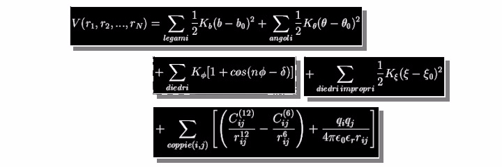
Classical Molecular Dynamics is based on a simplified description of the interactions among atoms of the molecular system. In this simplified model, electrons are not explicitly taken into account. Still, their effect is implicitly described by an effective potential ( or force field) that describes the atomic interactions. An example of force field potential, used in most Molecular Dynamics simulation programs, is shown in the slide. The first two terms describe bond stretching and bending in the harmonic approximation. The second two expressions model the torsion potential (used, for example, to describe a double bond) and the improper dihedral (used to constraint atoms to particular geometric, for example, to keep planar aromatic rings), respectively.
Finally, the last two terms describe the nonbonded interactions, namely the van der Waals and the electrostatic interactions. All the constants present in the potential V are determined from experimental data (e.g., the force constants could be derived from the spectroscopic Infrared red measurements) o quantum mechanical calculations (e.g., partial charges), for this reason, the force field is defined as semi-empirical.
The derivative of V provides the classical forces acting on the single atoms. The physics for the next steps of the method is known since more than 300 years ago. In fact, given the positions and velocities of atoms at time t, it is possible, by integrating the Newton equation, to obtain new coordinates positions and velocities at the time t+dt (where it is the numerical integration step). In this way, it is possible to generate the trajectory of each atom in our molecular system. The analysis of these trajectories provides a mine of important information on the simulated system.
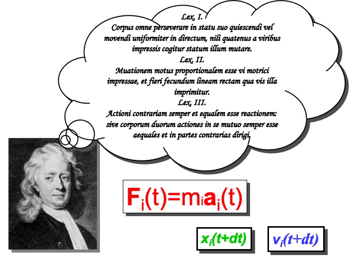
Isaac Newton. Philosophiae Naturalis Principia Mathematica. London, 1686.
Some of this information can be compared with the available experimental data to validate the model, but most can be used to understand microscopic phenomena that can be difficult to observe experimentally.
The kind of information that we can retrieve from an MD experiment can be classified as follows:
- Structural ( e.g., conformational change in proteins o nucleic acid, property of the material)
- Thermodynamics (e.g. solution enthalpy, heat capacity, free energies)
- Dynamics ( e.g. diffusion and viscosity coefficients)
In the following table, the history of applying MD simulation methods to study the system of biological interest is briefly reported. The first simulation of a biological macromolecule was performed in 1977 by Andrew McCammon et al. (J.A. McCammon, B.R. Gelin, and M. Karplus, Nature 267 (1977), 585). The simulated protein was the Bovine Pancreatic Trypsin inhibitor, and the simulation was performed in vacuo. Nowadays, simulations of this time scale are not performed anymore. In 1998, the microsecond barrier was overcome by Duan and Kollman (Yong Duan and Peter A. Kollman Science 1998 October 23; 282: 740) on a protein of 36 residues. However, this record did not last not long.
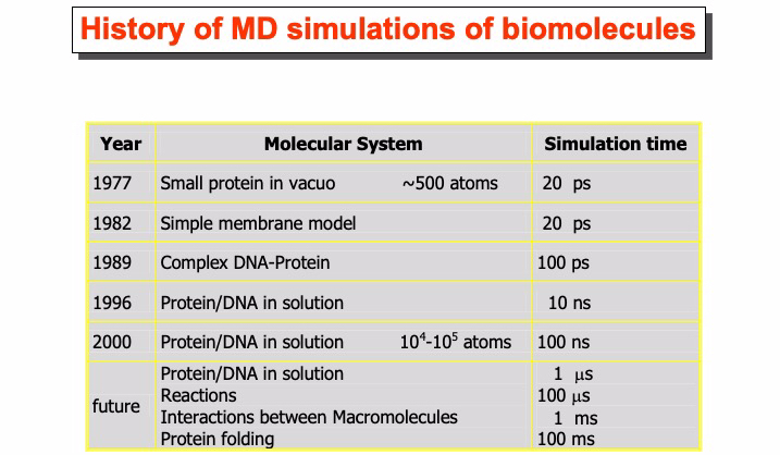
In fact, the semi-empirical force field allows the study of large systems and for time scales that are limited by the performance of the available computer architectures. The progressive increase of computer power makes the future development of this technique exciting and challenging. Nowadays, dedicated hardware such as the supercomputer Anton of the de Shaw research enterprise can perform millisecond long MD simulations matching the time scale of phenomena as protein folding and aggregation. The achievements of such a target turned MD from an academic research method to a practical and powerful digital nanoscope that allows making essential steps in understanding functional molecular biology.
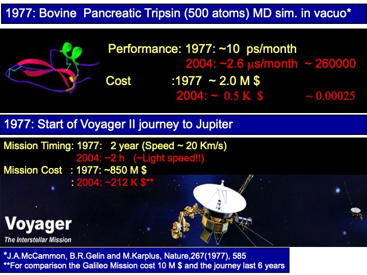
To understand the impact of the computer on the MD simulation method, in my lesson, I show the following analogy to my students. The first simulation of a protein was performed in 1977 (see reference, I will talk more about in another article), and in the same year, Voyager II started his journey to Jupiter. The simulations consisted of a system of ~500 atoms. The simulation ran on the best supercomputer of that time, which would cost around 2 million dollars, run at ~10 ps /month. Today the same simulation on a PC would run in one month 3 microseconds on a piece of equipment 4000 times less expensive. If the same would apply to the space mission, a mission to Jupiter would cost in 2004 only 200000 dollars and will reach the planet in a couple of hours instead of the two years required!
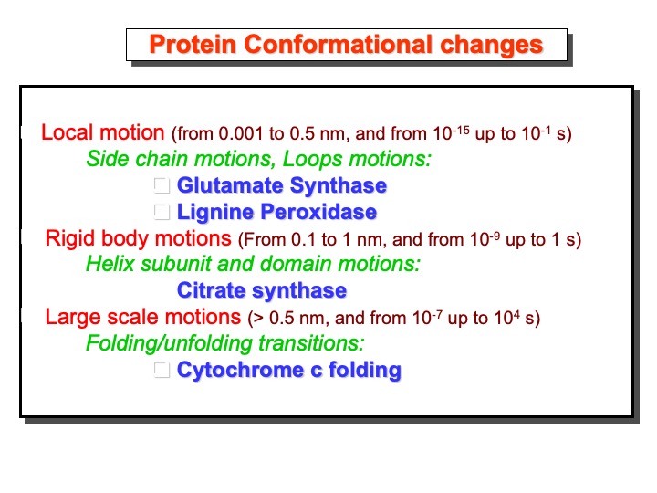
The free energy landscape of proteins is exemplified pictorially as a multidimensional corrugated funnel. The burrow of the funnel is where the protein chain falls during its folding process. The bottom of the funnel, the native or folded state of the protein, is also a sculptured landscape made of hills and valleys of different sizes and deep, representing the less extensive variations that the protein undergoes in its native state. The heights of hill peaks and passes represent the barriers among conformation states. From the kinetic theory, we can estimate the so-called first-passage time that gives the order of magnitude for the time of these processes. Some examples of these times scales are shown in the slides below with some proteins from my research studies.
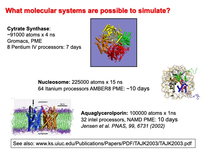
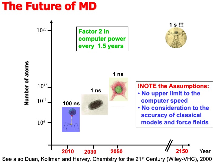
At the time of my talk (2004), I exemplified in the following graph, the range in time and scale of common systems simulation with MD.
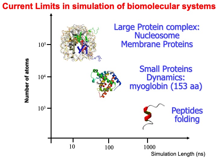
I also reported some more specific examples in this slide. Today, the time scale has much improved by one or even two orders of magnitude, depending on the computer hardware available.
Duan, Kollman, and Harvey, have predicted in a book chapter contributed in the collection Chemistry for the 21st Century that in the second half of this century, we would be able to simulate the entire cycle of replication for the bacterium E. Coli (t=1000 s, 
Some example of MD simulations
Lignin is the most abundant organic material on earth after cellulose. It is an essential component of higher plants, giving them rigidity, water-impermeability, and resistance against microbial decay. White-rot fungi are the only organisms able to mineralize lignin efficiently to carbon dioxide and water through processes initially catalyzed by extracellular enzymes. Lignin peroxidase (LiP), a heme-containing glycoprotein isolated from the ligninolytic cultures of the white-rot fungus Phanerochaete chrysosporium, is one of those enzymes capable of performing the oxidative depolymerization of lignin via an electron transfer (ET) mechanism.
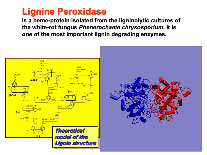
The enzyme is constituted by two identical monomers (blue and red in the picture), each containing a single iron protoporphyrin IX prosthetic group, two calcium ions, and four disulfide bonds. Each monomer consists of 344 amino-acid residues. In the picture, the protein is shown in a cartoon representation. In this representation, alpha-helices are shown as cylinders and strands as ribbons.
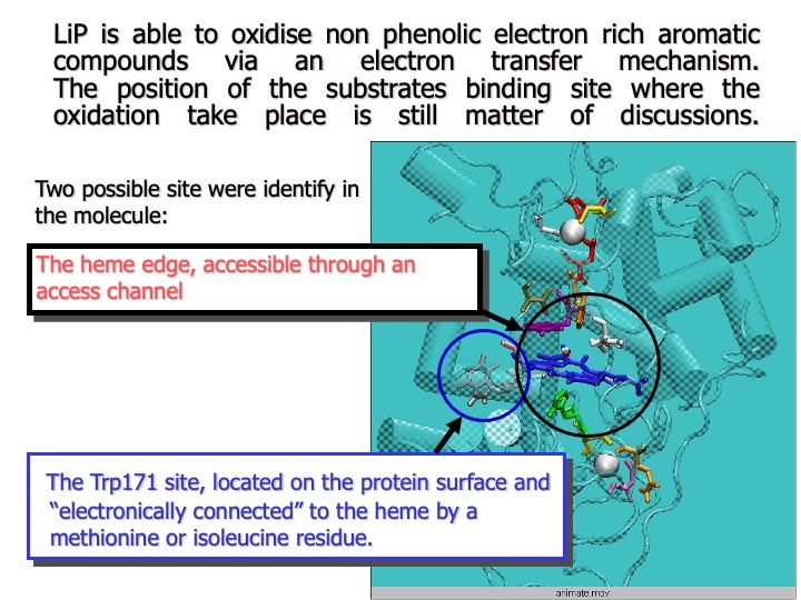
Very little is known about the substrate-binding site of LiP, and the pathway of electron flux from the substrate to the oxidized heme is still a matter of discussion.
The analysis of LiP crystal structure showed that both the active site and the substrate access channel appear almost inaccessible, compared to those of other peroxidases, and direct interaction between the enzyme active site and a substrate seems quite tricky. Thus, it has been proposed and generally accepted that small aromatic molecules, such as veratryl alcohol (3,4-dimethoxybenzyl alcohol, VA), a LiP natural substrate, are oxidized at the heme edge via a long-range ET.
Recently, it has also been suggested that VA might be oxidized via an ET mediated by the LiP surface residue Trp171 (beta-hydroxytryptophan, HTR), a hypothesis based on the observation that the mutation of this residue led to the loss of enzymatic activity toward VA oxidation. However, the pictures described above seem to be contradicted by other studies of kinetic activity.
Therefore, it is interesting to investigate the protein behavior in detail to better understand its structure and its dynamical properties in solution. Furthermore, molecular dynamics simulations supply a great deal of information regarding the stability of non-covalent interactions in water and the mobility of the amino-acidic residues within the protein frame. In fact, MD simulations provide a reliable model of macromolecules’ structural and dynamical behavior in a solution that might be different from the static picture of the protein obtained from its crystal structure. For these purposes, a 5 ns MD simulation of the native enzyme, the first long MD simulation on LiP, has been performed.
The starting structure for simulations was taken from the 0.17-nm resolution refined x-ray LiP crystal structure (Brookhaven Protein Data Bank, PDB code 1QPA). Only one monomer was used for the simulations. The protein was solvated in a periodic rectangular box with water of size 5.8×6.7×7.9 nm, large enough to contain the protein and 0.75 nm of solvent on all sides. Since the system has a total charge of 15, sodium counter-ions were added to neutralize the box charge. The resulting system was formed by the protein, approx. 8700 water molecules and 15 sodium ions, for a total of approx. 29,000 atoms. During the simulations, the temperature of the system was maintained constant to 300 K.
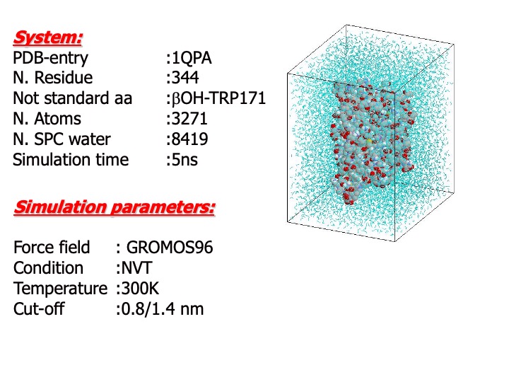
A time step of 2 fs for the integration of the motion equation was used.
The nonbonded interactions (electrostatic and van der Waals) were calculated using the cut-off method. The non-bonded interactions are proportional to the square of the number of atoms present in the system. To limit the number of calculations required, a cut-off method generally is used. It is based on the fact that the van der Waals and in less extend, electrostatic became negligible over a certain distance. Therefore, if each atom interacts only with other ones within a sphere of radius r (the cut-off radius), the total number of nonbonded interactions is drastically reduced.
The initial velocities of all atoms were taken from a Maxwellian distribution at the desired initial temperature.
Finally, all the MD runs and analyses of the trajectories were performed using the GROMACS software package (www.gromacs.org).
The primary analysis concerning the deviation of the protein structure regarding the initial reference structure is usually done in terms of root mean square deviation (RMSD) and radius of gyration (Rg). The first one (bottom formula on the slide) provides a global indication of the total deformation from the reference structure (usually the crystallographic one) of the configurations and the simulation. In the formula, r and 

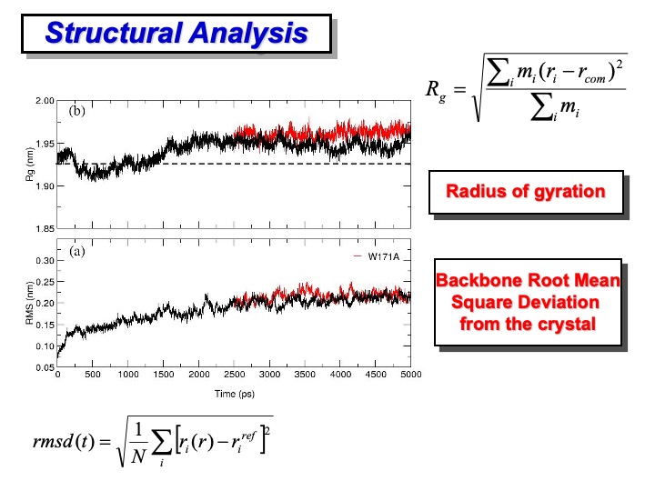
The RMSD of LiP backbone atoms relative to the crystal structure is shown in plot (a) on the slide. The protein atoms did not significantly deviate from the crystal structure, and the backbone RMSD is stabilized to an average value of 0.2 nm. Although the RMSD appears to rise slightly even after 1.5 ns, the fluctuation amplitudes obtained are relatively small. In plot (b), the gyration (Rg) of the protein along the simulation is reported. The average value, 1.95 nm, in the last 3 ns shows a slight deviation from the crystallographic one (1.925 nm, dashed line), which indicates a negligible crystallographic packing effect and a slight influence of the second monomer on the overall enzyme stability.
The active site residues and the calcium-binding sites are well conserved in a different type of peroxidase. Therefore it is crucial to analyze the change in its configuration occurring during the simulation. This evaluation is essential to check the correctness of the simulation itself. If significant and unexpected changes happen in this region, it is more likely that the force field or the stimulation protocol is incorrect.
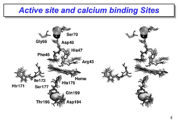
The analysis of the MD simulation revealed that in the active site, these key residues essentially maintained the conformation they have in the crystal structure; in fact, the RMSD of the active site residues is 0.13 nm. In particular, their hydrogen-bond network is retained and persisted during the simulation. Furthermore, the superimposition shown in the picture of the active site in the x-ray LiP crystal structure (bold line) with different frames from the simulation (grey lines) displays a very similar orientation of all the amino-acidic residues in the active site considered necessary for LiP activity, confirming that this protein area is very rigid.
The same picture shows that all the residues coordinated to both calcium ions do not deviate from their crystal orientations, thus indicating that this microenvironment is firmly conserved in solution. These results are following the expectation that the interactions between the calcium ions and the protein are essential to maintain the structure of the active site and, therefore, the enzymatic catalytic activity.
To provide a more detailed description of the deformation of the protein residues, the backbone RMSD per residue is shown in the lower plot on the slide—this type of analysis evidence the average deviation of each residue from the reference crystallographic structure. Differently from the previous RMSD, here, the average is done over time. The cyan bands indicate the regions of the protein where alpha-helix are located. The protein fragments having the most significant deviation are colored in red on the crystal structure representation on the right side. It is clear from this representation that the amplest variations do not involve residues forming structurally essential regions. In particular, the residues showing the largest displacements are those in the C- and N-termini of the protein, regions characterized by a low structural organization. Moreover, other residues that experience a large displacement are those forming loops mainly located on the LiP surface. From all these graphics, it is evident that the enzyme mostly retained the overall backbone structure in the simulation course.
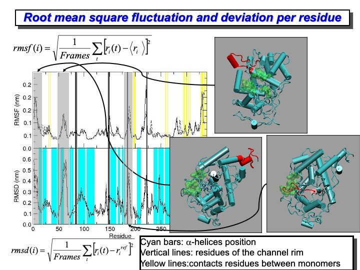
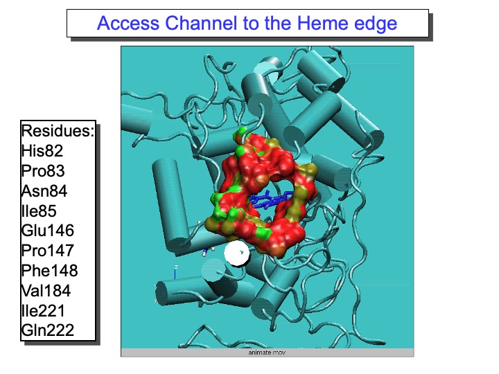
It is also interesting to quantify the mobility of each residue (or part of it) to identify the most flexible regions of the protein. The Root Mean Square Fluctuation (RMSF) provides this kind of information, and it is calculated using the formula reported in the upper part of the slide. The formula average over the simulation time, the deviation of each residue from the average structure of the protein. In the upper panel of the graph in the slide, the RMSF for the LiP is reported. It is evident the correspondence between large RMSD and the high RMSF values. The yellow lines indicate the residues located at the interface of the two monomers. The two monomeric LiP units are not covalently linked, but they are in contact through one loop (from residue 292 to 299 and 326 to 332), which is quite flexible during the simulation. Finally, the black lines indicate the position of the residue located on the rim of the access channel to the heme edge (green surface in the pictures on the right). In this case, some of the residues are located in the region of high mobility and deformation.
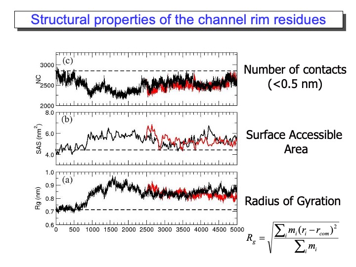
The most exciting and surprising results came from the MD data analysis for the residues forming the substrate access channel to the heme. LiP heme is not in direct contact with the solvent but is located at the bottom of a fissure, recessed from the protein surface. A cleft, found in heme peroxidases but with variable sizes, provides access to it from the surface. Compared to other peroxidases, like cytochrome C peroxidase and Coprinus cinereus peroxidase, LiP has bulkier residues whose side chains occupy, in part, the entrance, so that direct interaction of large substrates with the heme in the active site appears highly unlikely. Thus, one of the still-open questions regarding LiP activity is how a substrate is oxidized by this enzyme. In the upper graph of the next slide, the analysis of the Rg of the amino-acid residues forming the access channel, the solvent-accessible surface of this area and the number of contacts (NC) between these residues, reported (black line). The variations of these properties during the time of the simulation are correlated. Accordingly, an increase in Rg corresponded to the rise in the solvent-accessible surface and decreased NC, indicating that the access channel is increasing its opening.
Thus, this analysis pointed out the occurrence of conformational changes of the protein access channel, suggesting that a substrate can enter the solution channel. The enlargement of the heme access channel is pictorially represented in the bottom Figure, where the x-ray crystal structure (0 ps) and different frames extracted from the simulation are reported. Hence, a relaxation of the protein occurs in solution, demonstrating that the picture obtained from the x-ray crystal structure represents a lower limit.

So far, we have shown that the access channel to the heme edge change in solution by enlarging his rim compared to the crystal structure. But is it now possible for the substrate to reach the heme edge? Unfortunately, VA’s spontaneous (diffusive) entrance into the LiP active site access channel would require a timescale too long to be observed by a typical MD simulation. For this reason, we have used the docking method called Steered Molecular Dynamics (SMD) to accelerate this process. However, it is essential to point out that SMD provides only qualitative information on the docking process that is sufficient to assess energy barriers. Quantitative results would require calculating the potential mean force along the docking pathway, but this is computationally very expensive.
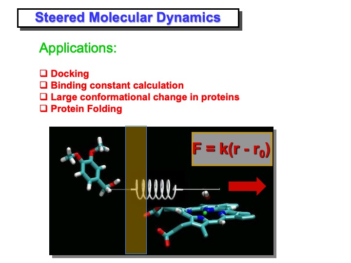
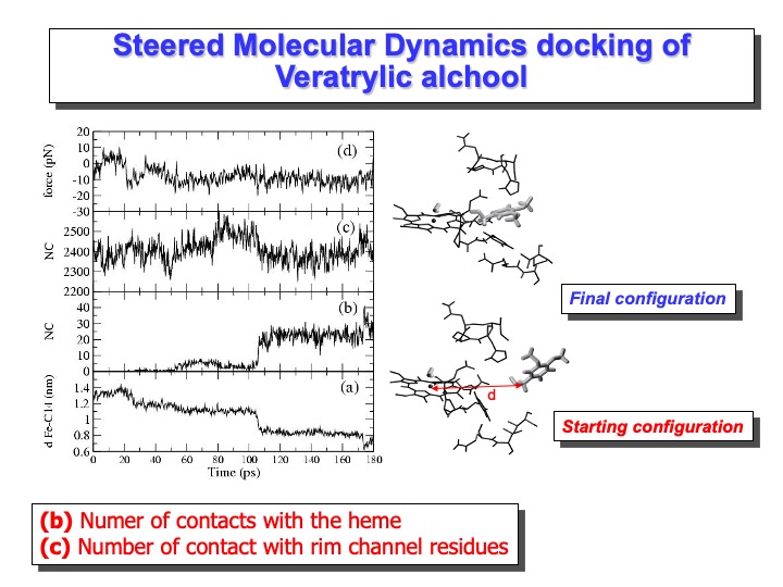
The steered molecular dynamics (SMD) method is used to study different types of non-equilibrium processes: ligand binding and unbinding to proteins, domain motion, and protein folding. SMD docking provides a means to accelerate those processes by applying external forces that lower the energy barrier and drive the ligand to the active site in a nanosecond timescale. In this simulation, VA was pulled toward the iron. This was performed by applying a harmonic restraint between the benzylic carbon of VA and a point moving at constant velocity along a line connecting the carbon with the iron in the heme (see slide above). At starting VA molecule was positioned in front of the access channel by manual docking, replacing a few overlapping water molecules. After a preliminary minimization and equilibration procedure, in which VA molecule was kept at a fixed distance from the heme-iron atom, the SMD simulation was started.
The length of the SMD simulation was 180 ps. The starting distance between the Fe and the VA benzylic C atom (C14) was 1.4 nm (see graph (a) on the slide), and the starting configuration is reported on the right side of the Figure. After 180 ps this distance decreases to 0.75 nm. The curve in graph (a) shows two steps in correspondence of 25 ps and 100 ps. The second step corresponds to a situation in which VA is close to the heme edge, as shown in graph (b), where the number of contacts of VA with heme atoms (within 0.4 nm) is reported. The value of the constraint force, graph (d), fluctuates around 0, indicating the presence of favourable interactions across the access channel. Finally, the lack of channel residues’ perturbation by the incoming VA molecule is shown in graph (b), where the number of contacts among the residues forming the access channel is reported. The number of contacts remains similar to that observed in the simulation. Thus, it would appear that VA could easily approach the heme edge up to a distance of 0.4 nm without disturbing the protein. The final configuration is reported on the right side of the slide.
Glutamate synthases
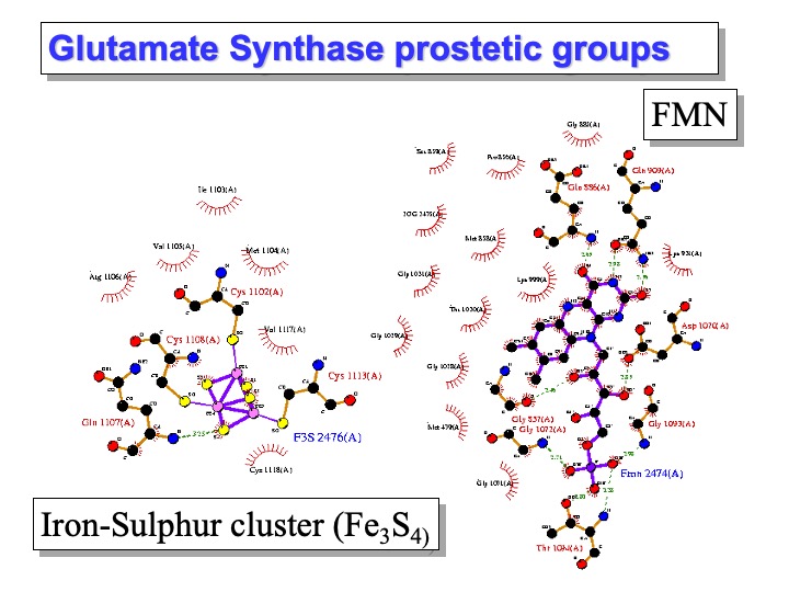
Glutamate synthases (GltS) are complex iron-sulfur flavoproteins that catalyze the reductive transfer of the L-glutamine (L-Gln) amide group to the (C2) carbon of 2-oxoglutarate (2-OG), yielding two molecules of L-glutamate (L-Glu). GltS are found in bacteria, yeast, and plants where they form with glutamine synthetase, an essential pathway for ammonia assimilation, and fall in one of three classes: the bacterial NADPH-dependent GltS (NADPH-GltS), the plant-type ferredoxin-dependent species (Fd-GltS), and the eukaryotic NADH- dependent enzyme (NADH-GltS).
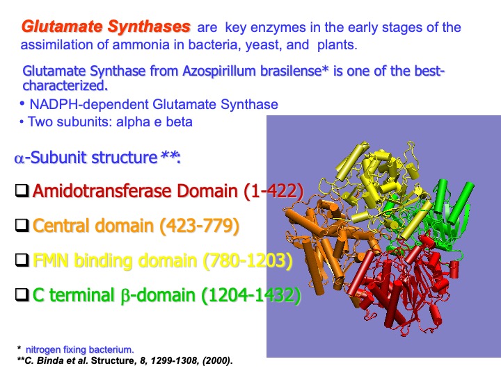
Azospirillum Brasiliense GltS is the bacterial enzyme form prototype, which depends on NADPH as the physiological electron donor. The stable and catalytically active 
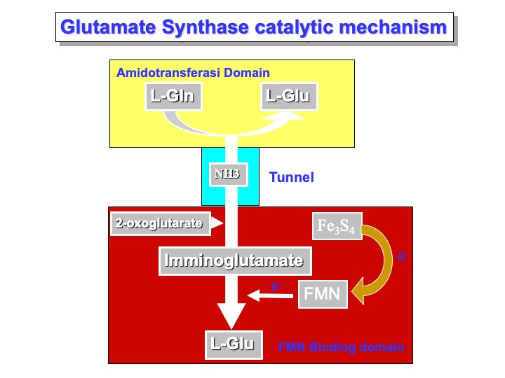
In the Glutamine Synthase, two active sites are present. A molecule of L-Glutamine binds to the AMD domain active site. As a molecule of 2-oxoglutarate binds the FMN binding domain active site, the hydrolysis reaction occurs, and a molecule of ammonia is released. Simultaneously (or before), the ammonia tunnel that passes through the center domain enlarges the rim in the proximity of the AMD domain, allowing the ammonia to diffuse to the FMN active site. Here, the reaction with 2-oxoglutarate occurs with the formation of a molecule of 2-iminoglutarate. In the meantime, the FMN molecule is reduced by the iron-sulfur cluster and can chemically reduce imminoglutarate and form a molecule of L-glutamic acid.
MD simulations were performed starting from the crystallographic coordinates of a-GltS A-chain (PDB code 1EA0 ). Two simulations were performed. In one simulation, the ligands present in the crystal structure were removed, and the free enzyme was simulated. In the other, an L-glutamine and a 2- oxoglutarate molecule were kept in their relative binding positions.
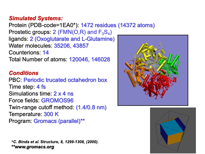
The simulation conditions were similar to those already shown for the Lignin peroxidase. To save computational time, a periodic truncated octahedron box was used. In this way, the number of water molecules necessary to solvate the protein is substantially less than in the case of a cubic box. Furthermore, for the same reason, a longer integration time step was used. However, even with these tricks, the resulting size of the system was considerably large. Thus, it was necessary to perform the simulations on parallel computers. In this way, the computational demand is distributed on more processors, speeding up the computational time.
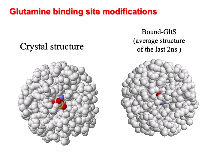
A comparison of the simulated -GltSfree and -GltSbound structure shows that the presence of ligand strongly influences the two simulated system dynamics. For example, a close inspection of the amidotransferase active site, evidence that the binding cavity in the presence of the L-glutamine turns out to be partially protected from the solvent due to the loop 263-271 that water molecules can penetrate the cavity. In the Figure, the amidotransferase binding cavity at the beginning (left) and averaged over the last 2 ns (right) are shown. L-Glutamine is represented in colour.
Another intriguing effect concerns the ammonia tunnel connecting the AMD domain and the FMN domain.
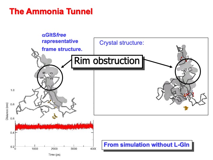
As previously discussed, the ammonia molecule produced at the L-Gln binding (glutamine amidotransferase ) site of GltS must reach the enzyme synthase site to add to 2-OG C(2) position to form the 2-iminoglutarate intermediate of the synthase reaction. In the crystal structure of a-GltS in complex with L-MetS and 2-OG an obstructed tunnel connects the two catalytic sites, about 31 Å apart. Backbone atoms of residues 507-508 of the central domain and 976-977 of the flavin binding domain form the obstruction. The distance between the centers of mass of 
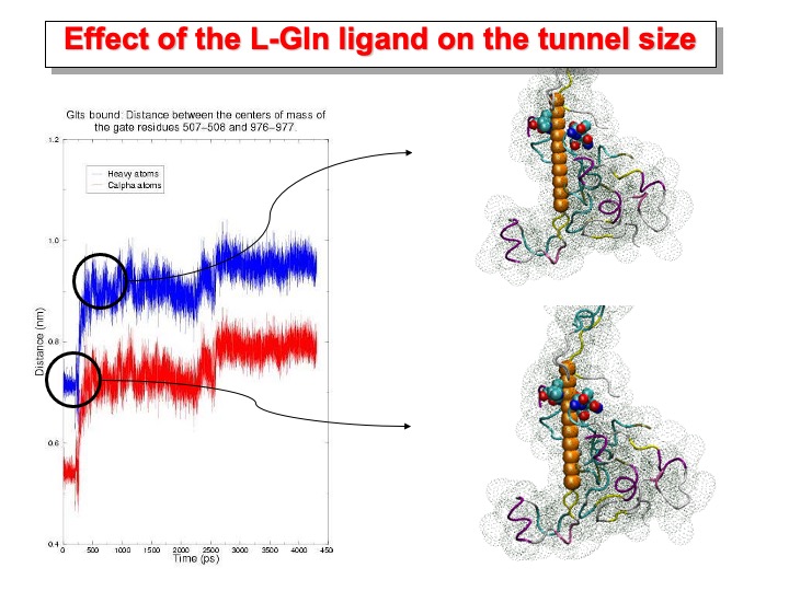
In the-GltSbound, the binding of the ligand to the polypeptide produces the opening of the passageway. The distance between the centers of mass of Ca of residues 507-508 and 976-978 varies between 0.67 and 0.87 nm (plot in red). The gap is large enough to allow the channeling of NH3 from the amidotransferase active site to the synthase site where 2-OG is bound. In the pictures on the right side, the structure before and after the tunnel opening is shown. The tunnel is schematically represented with a sphere having the radius of an ammonia molecule, and only a portion of the protein is shown as ribbon and dotted surface. The residues on the rim of the tunnel are represented as colored spheres.