The Taylor series is a mathematical tool that, sometimes, it is not easy to immediately grasp by freshman students. In this blog, I will give a short review of it giving some examples of applications.
Who is Mr. Taylor?
Brook Taylor (1685 – 1731) was a 17th-century British mathematician. He demonstrated the celebrated Taylor formula, the topics of this blog, in his masterwork Methodus Incrementorum Directa et Inversa (1715). For more information, just give a read to the following wiki page.
The Taylor Theorem
Let k ≥ 1 be an integer and let the function f : R → R be k times differentiable at the point a ∈ R. Then there exists a function hk : R → R such that

The polynomial in the series is called k-th order Taylor polynomial:

The difference of the series with respect the funzion $f(x) is given by the relation
which gives the error in the approximation of 

The MacLaurin Series
The work developed by Taylor was promtly adopted by the Scottish mathematician Colin MacLaurin (1698–1746) that used Taylor series to characterize maxima, minima, and points of inflection for infinitely differentiable functions in his Treatise of Fluxions. For his contributions to the development of this important mathematical tool, when the general expression given is used with 
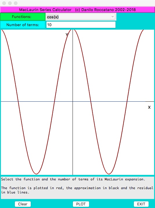
An example: the cos(x) expansion
The MacLaurin series for the 

In the following panels the expansion for k=1, 2, 3, 6 and 10 terms are reported (see appendix for the program). The function is shown in red, the series in black and the difference in blue colour.


Some examples of MacLaurin series
Some of commonly used Maclaurin series include:


You can use the program in the Appendix I to graphically explore the MacLaurin series of some these functions.
Multivariate Taylor Series
The Taylor series can be easily generalized to the multivariate functions. For example let consider the 

![f(x,y)=f(a,b)+f_x(a,b)(x-a)+f_y(a,b)(y-b)+\frac{1}{2!}\left[f_{xx}(a,b) (x-a)^2+ 2f_{xy}(a,b) (x-a)(y-b)+f_{yy}(a,b)(y-a)^2\right]+\frac{1}{3!}\left[f_{xxx}(a,b)(x-a)^3+3f_{xxy}(a,b)(x-a)^2(y-b)+3f_{xyy}(a,b)(x-a)(y-b)^2 +f_{yyy}(a,b)(y-a)^3\right]+\frac{1}{4!}\left[f(x,y)_{xxxx}(x-a)^4+4f_{xxxy}(x-a)^3(y-b)+6f_{xxyy}(x-a)^2(y-b)^2+f_{yyyx}(x-a)(y-b)^3 + f_{yyyy}(y-b)^4\right]](https://s0.wp.com/latex.php?latex=f%28x%2Cy%29%3Df%28a%2Cb%29%2Bf_x%28a%2Cb%29%28x-a%29%2Bf_y%28a%2Cb%29%28y-b%29%2B%5Cfrac%7B1%7D%7B2%21%7D%5Cleft%5Bf_%7Bxx%7D%28a%2Cb%29+%28x-a%29%5E2%2B+2f_%7Bxy%7D%28a%2Cb%29+%28x-a%29%28y-b%29%2Bf_%7Byy%7D%28a%2Cb%29%28y-a%29%5E2%5Cright%5D%2B%5Cfrac%7B1%7D%7B3%21%7D%5Cleft%5Bf_%7Bxxx%7D%28a%2Cb%29%28x-a%29%5E3%2B3f_%7Bxxy%7D%28a%2Cb%29%28x-a%29%5E2%28y-b%29%2B3f_%7Bxyy%7D%28a%2Cb%29%28x-a%29%28y-b%29%5E2+%2Bf_%7Byyy%7D%28a%2Cb%29%28y-a%29%5E3%5Cright%5D%2B%5Cfrac%7B1%7D%7B4%21%7D%5Cleft%5Bf%28x%2Cy%29_%7Bxxxx%7D%28x-a%29%5E4%2B4f_%7Bxxxy%7D%28x-a%29%5E3%28y-b%29%2B6f_%7Bxxyy%7D%28x-a%29%5E2%28y-b%29%5E2%2Bf_%7Byyyx%7D%28x-a%29%28y-b%29%5E3+%2B+f_%7Byyyy%7D%28y-b%29%5E4%5Cright%5D&bg=ffffff&fg=444444&s=0&c=20201002)
An example
Let see as an example the function
The fourth order Taylor series is given by
![f(x,y)= F(a,b)+\sin(x)\cos(y)(x-a) + \cos(x)\sin(y)(y-b)+\frac{1}{2!}\left[-\cos(x)\cos(y) (x-a)^2+ 2\sin(x)\sin(y)(x-a)(y-b) -\cos(x)\cos(y)(y-b)^2\right] + \frac{1}{3!}\left[ \sin(x)\cos(y)(x-a)^3+3\cos(x)\sin(y)(x-a)^2(y-b)+3\sin(x)\cos(y)(x-a)(y-b)^2+\cos(x)\sin(y)(y-b)^3\right] + \frac{1}{4!}\left[\cos(x)\cos(y)(x-a)^4-4\sin(x)\sin(y)(x-a)^3(y-b)+6\cos(x)\cos(y)(x-a)^2(y-b)^2-\sin(x)\sin(y)(x-a)(y-b)^3 + \cos(x)\cos(y)(y-b)^4\right]](https://s0.wp.com/latex.php?latex=f%28x%2Cy%29%3D+F%28a%2Cb%29%2B%5Csin%28x%29%5Ccos%28y%29%28x-a%29+%2B+%5Ccos%28x%29%5Csin%28y%29%28y-b%29%2B%5Cfrac%7B1%7D%7B2%21%7D%5Cleft%5B-%5Ccos%28x%29%5Ccos%28y%29%C2%A0%28x-a%29%5E2%2B+2%5Csin%28x%29%5Csin%28y%29%28x-a%29%28y-b%29+-%5Ccos%28x%29%5Ccos%28y%29%28y-b%29%5E2%5Cright%5D+%2B+%5Cfrac%7B1%7D%7B3%21%7D%5Cleft%5B+%5Csin%28x%29%5Ccos%28y%29%28x-a%29%5E3%2B3%5Ccos%28x%29%5Csin%28y%29%28x-a%29%5E2%28y-b%29%2B3%5Csin%28x%29%5Ccos%28y%29%28x-a%29%28y-b%29%5E2%2B%5Ccos%28x%29%5Csin%28y%29%28y-b%29%5E3%5Cright%5D+%2B+%5Cfrac%7B1%7D%7B4%21%7D%5Cleft%5B%5Ccos%28x%29%5Ccos%28y%29%28x-a%29%5E4-4%5Csin%28x%29%5Csin%28y%29%28x-a%29%5E3%28y-b%29%2B6%5Ccos%28x%29%5Ccos%28y%29%28x-a%29%5E2%28y-b%29%5E2-%5Csin%28x%29%5Csin%28y%29%28x-a%29%28y-b%29%5E3+%2B+%5Ccos%28x%29%5Ccos%28y%29%28y-b%29%5E4%5Cright%5D+&bg=ffffff&fg=444444&s=0&c=20201002)
In the case of the MacLaurin series 
![f(0,0)= 1-\frac{1}{2}\left[(x)^2 + (y)^2\right]+\frac{1}{24}\left[ x^4 +x^2y^2+y^4\right]](https://s0.wp.com/latex.php?latex=f%280%2C0%29%3D+1-%5Cfrac%7B1%7D%7B2%7D%5Cleft%5B%28x%29%5E2+%2B+%28y%29%5E2%5Cright%5D%2B%5Cfrac%7B1%7D%7B24%7D%5Cleft%5B+x%5E4+%2Bx%5E2y%5E2%2By%5E4%5Cright%5D&bg=ffffff&fg=444444&s=0&c=20201002)
In Figure 2, the function and its second order approximation approximation is shown.

In Figure 3, the MacLaurin surface including also the 4th order approximation terms is shown. Note that the third order expansion does not contribute to the series since all the third order partial derivatives calculated at (0,0) are equal to zero.

APPENDIX
A program to explore MacLaurin series of functions in one variable
The following program in TCL/TK language allows to calculates and compares the first terms of a MacLaurin series of some transcendent functions.
#! /bin/sh
# the next line restarts using wish \
exec wish "$0" "$@"

# root is the parent window for this user interface

package require Tk

wm title . ""
tk_setPalette cyan3

# Define some variables
# this treats "." as a special case
set root "."

set base ""
set maxX 500
set maxY 500
set width  0
set height 0
set midX   0
set midY   0

set rmin -1.0
set rmax 1.0
set ymax   5.
set ymin  -5.
set np 500
set nt   1
set lfuncts "exp(x)"

# Define global variables

global nt width height dcc lfuncts maxX maxY


#############################################################################
## Procedures
# Some of the procedure are adapted from: http://wiki.tcl.tk/15073
#
#############################################################################

proc fact n {expr {$n<2? 1: $n * [fact [incr n -1]]}}


proc ClrCanvas {w } {
    global dcc
    global rmin rmax width height ymax ymin midX midY

    $w delete "all"
    set dcc 0
    DrawAxis $w
}

proc DrawAxis {w} {

    global rmin rmax  width height ymax ymin midX midY maxX maxY

    set midX  [expr { $maxX  / 2 }]
    set midY  [expr { $maxY   / 2 }]
    set incrX [expr { ($maxX -50) /10 }]
    set incrY [expr { $maxY   /11 }]
    #    puts "$midX $midY"

    $w create line 0 $midY  $width   $midY  -tags "Xaxis"  -fill black -width 1
    $w create line $midX 0  $midX $height  -tags "Yaxis" -fill black -width 1
    $w create text [expr $midX-20] 20 -text "Y"
    $w create text [expr $width-20]  [expr $midY+20]  -text "X"
}

proc DrawFn w {

    #
    # Plot the sunflover florets
    #

    global cc np nt
    global rmin rmax  width height ymax ymin midX midY lfuncts maxX maxY

    ClrCanvas .cv
    #    puts "$lfuncts"
    if {$lfuncts  == "exp(x)"} {
        set rmin -1.0
        set rmax 1.0
        set ymax   5.
        set ymin  -5.
} else {
    set rmin -3.1415*2
    set rmax  3.1415*2
    set ymax   1.
    set ymin  -1.
}
if {$lfuncts == "sinh(x)"} {
    set rmin -3.1415/2
    set rmax  3.1415/2
        set ymax   3.
        set ymin  -3.
}


set divy [expr ($ymax-$ymin)/$maxY   ]
set divx [expr ($rmax-$rmin)/$maxX   ]
set asp_ratio 1.
set x $rmin

DrawAxis $w
for { set n 1 } { $n <= $np } { incr n 1 } {

    set x  [expr $x+$divx]
    set xp [expr $midX+ $x/$divx]

    if {$lfuncts  == "exp(x)"} {
        set y  [expr exp($x)]
        set ys 1.0
        for { set m 1} {$m <= $nt} { incr m 1} {
            set ys [expr $ys + pow($x,$m)/([fact $m])]
}
}
if {$lfuncts  == "sin(x)"} {
    set y  [expr sin($x)]
    set ys 0
    for { set m 0} {$m <= $nt} { incr m 1} {
        set kk [expr 2*$m+1]
        set sign [expr pow(-1,$m)]
        set ys [expr $ys + $sign*pow($x,$kk)/([fact $kk])]
}
}
if {$lfuncts  == "cos(x)"} {
    set y  [expr cos($x)]
    set ys 1
    for { set m 1} {$m <= $nt} { incr m 1} {
        set kk [expr 2*$m]
        set sign [expr pow(-1,$m)]
        set ys [expr $ys + $sign*pow($x,$kk)/([fact $kk])]
}
}
if {$lfuncts  == "atan(x)"} {
    set y  [expr atan($x)]
    set ys 0
    for { set m 0} {$m <= $nt} { incr m 1} {
        set kk [expr 2*$m+1]
        set sign [expr pow(-1,$m)]
        set ys [expr $ys + $sign*pow($x,$kk)/($kk)]

}
}
if {$lfuncts  == "sinh(x)"} {
    set y  [expr sinh($x)]
    set ys 0
    for { set m 0} {$m <= $nt} { incr m 1} {
        set kk [expr 2*$m+1]
        set ys [expr $ys + pow($x,$kk)/($kk)]
}
}

set r [expr $y-$ys]
set yp [expr $midY- $y/$divy*$asp_ratio]
set ysp [expr $midY- $ys/$divy*$asp_ratio]
set re  [expr $midY- $r/$divy*$asp_ratio]

if {$n > 1} {
    .cv create line $x0 $y1  $xp $yp   -tags "Exact"  -fill red    -width 2
    .cv create line $x0 $y2  $xp $ysp  -tags "approx" -fill black  -width 1
    .cv create line $x0 $y3  $xp $re   -tags "resid"  -fill blue   -width 1
}
set y1  $yp
set y2  $ysp
set y3  $re
set x0  $xp

}

}

###############################################################################################
#
# Main with the setup up of the GUI
###############################################################################################

# Row 1
label $base.label#12 \
-background magenta -padx 64 -relief raised -text {MacLaurin Series Calculator   (c) Danilo Roccatano 2002-2018}

# Row 2

label $base.label#1 -background green -relief groove -text "Functions:  "
ttk::combobox $base.functions -textvariable lfuncts

.functions configure -values [list exp(x) sin(x) cos(x) atan(x) sinh(x)]

# row 3

label $base.terms  -background cyan -relief groove -text "Number of terms:" -bg cyan
entry $base.nt    -cursor {} -textvariable nt  -bg white

# row 5

canvas $base.cv -bg white -height $maxY -width $maxX

# row 6

button  $base.plot -text PLOT    -command { DrawFn .cv }
button  $base.b0   -text "Clear" -command { ClrCanvas  .cv }
button  $base.b1   -text "EXIT"  -command { exit -1}

text $base.t -width 50 -height 5 -wrap word  -bg gray90

.t insert end "Select the function and the number of terms of its MacLaurin expansion.\n
The function is plotted in red, the approximation in black and the residual in blue lines."


#
# Add contents to grid
#

# Row 1

grid $base.label#12 -in $root	-row 1 -column 1  -columnspan 4 -sticky nesw
# Row 2
grid $base.label#1 -in $root	-row 2 -column 1 -sticky nesw
grid $base.functions -in $root	-row 2 -column 2 -sticky nesw

grid $base.terms  -in $root	-row 4 -column 1  -sticky nesw
grid $base.nt    -in $root	-row 4 -column 2  -sticky nesw

# Row 9 (Canvas)

grid $base.cv -in $root	-row 5 -column 1  -columnspan 4  -sticky nesw

# Row 10

grid $base.t    -in $root -row 6 -column 1 -columnspan 4  -sticky nesw

grid $base.b0 -in $root	        -row 7 -column 1
grid $base.plot -in $root	    -row 7 -column 2
grid $base.b1 -in $root	        -row 7 -column 4

# additional interface code

bind $base.nt <Return> {DrawFn .cv }

update

# end additional interface code

set width  [winfo width .cv ]
set height [winfo height .cv ]

DrawFn .cv


Pingback: La Serie di Taylor | Danilo Roccatano
Pingback: Calculus in a Nutshell: functions and derivatives | Danilo Roccatano