The Mighty Roto-Microscope

I am happy to announce our second Instructable project. Like the first one, it was a long-standing idea that was rolling in my mind for a long time. The current limited travelling mobility due to the COVID offered more time to develop this idea during my vacation. In a joyful collaboration with my son Leonardo, we managed to realize this useful device in a very short time.

This project aimed to develop a device that integrated with a cheap USB microscope allows taking 3D pictures of small samples. The project is meant to be an education STEM activity to learn using Arduino, 3D image reconstruction, and 3D printing by creating a useful piece of equipment for doing some exciting science activity. Like my previous project, it is also a moment to share good and educative time with my family and in particular, my elder son Leonardo that helped me in creating this instructable and evaluating the device as an enthusiastic STEM student. This time, also my lovely wife helps me to make a video of the assembly of the equipment!

The roto-microscope allows controlling the position of a simple USB microscope around the sample. This allows to take accurate pictures from different angles and not just from the top as in the traditional microscopes. This is not a new idea as there are professional microscopes. However, this device means to be affordable for a student and still provides some similar results and a lot of fun in building it. Other similar and excellent OpenSource projects are available (see, for example, the Ladybug microscope, the Lego microscope, and the OpenScan project), our project adds an additional option and I hope that you enjoy making it as we did!

If you find it an interesting device then instructions on how to build it are on our Instructable.

The Magic Sand Slicer

We have published for the first time a project on Instructables: a website specialised in publishing interesting DIY projects by an effervescent community of makers and educators.

The project is called the Magic-Sand Slicer and it is an education project initially conceived as a STEM activity to learn using Arduino, a 3D printer, and some exciting science. It is also a collaboration with my son Leonardo who helped me in evaluating the device as a STEM student. We have learned a lot together, and we want to share the results of this long journey. This project aims to create a device that automatically makes sections of a cylinder of easy-to-cut coloured material. That can be used for practising 3D image reconstruction of the coloured blogs hidden in the column. The so-called Magic-Sand (c), also known with other trademarks names, becomes suitable for this experiment.
What is the point of making pictures of thin layers of sand and then reconstructing it digitally? Is it just for the fun of it? It varies on who is using it. However, students and teachers from different disciplines (e.g. geology, biology, medical) can find it a helpful education device to practice with image reconstruction from the serial sections. It could also be of interest to a geologist interested in sedimentary material plasticity to study rock and the secrets it beholds, or to a process, engineering to emulate the packing of fine granular materials. Finally, an artist can make a fantastic program of unravelling magic forms generated by packing coloured sand. 

I was surprised that the project got so much interest in a very short time and I thank the Instructable community for their nice welcome! If you like to know more about the project (and try it!) then you can read our instructable here.

I also just realized that the Instructable was reviewed on the Arduino blog site by the Arduino team!

Seminar Series: Molecular Dynamics Simulation of Biomolecules

In this new series, I will post slides of seminars or lessons that I have delivered in the past years. Some of the reported information is updated, but still helpful. In some cases, I have added descriptions of the slide contents or references to other articles or the original paper where I describe my research results.
I hope you like the presentation, and remember to add your feedback and subscribe to have email notifications about my new blog posts.

In 1648, Isaac Newton published his first edition of the Principia Mathematica, one of the greatest scientific masterpieces of all time. On page 12 of this magnum opus, the famous three laws that bear his name and from which classical mathematical physics evolved are enunciated. More than 350 years after that publication, the same laws formulated to explain the motion of stars and planets remain valuable for us when trying to simplify the description of the atomic world. In the first decades of the last century, the birth of quantum mechanics marked the beginning of the detailed description of atomic physics. The equation of Schrödinger, to the same extent as Newton’s equations, allowed for the mathematically elegant formulation of the shining theoretical intuitions and the experimental data accumulated in the previous decades. Although this equation could be used in principle to describe any molecular system’s physicochemical behaviour, it is impossible to resolve analytically when the number of electrons is more than two. The invention of electronic computers after World War II facilitated the numerical solution of this equation for polyatomic systems. However, despite the continuous and rapid development of computer performance, the ab-initio quantum-mechanical approach to describe static and dynamic properties of molecules containing hundreds or even thousands of atoms, as for biological macromolecules, is still far from becoming a standard computational tool. This approach requires many calculations that can be proportional to N^{3-5}
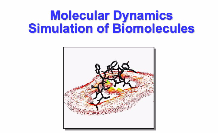
, where N is the total number of electrons in the system. It was clear that a reduction, using ad hoc approximations, of the description of the dynamic behaviour of atoms using a classic physics model would be necessary to overcome this problem. In the classical representation, the electrons on the atoms are not explicitly considered, but their mean-field effect is taken into account. Alder and Wainwright performed the first simulation of an atomic fluid using this approximation approximately 63 years ago (1957). They developed and used the method to study simple fluids by means of a model representing atoms as discs and rigid spheres. These first pioneer studies mark the birth of the classical molecular dynamics (MD) simulation technique. The successive use of more realistic interaction potentials has allowed obtaining simulations comparable to experimental data, showing that MD can be a valuable tool for surveying the microscopical properties of physical systems. The first simulations of this type were carried out by Rahman and Verlet (1964): in these simulations, a Lennard-Jones-type potential was used to describe the atomic interactions of argon in the liquid state. Another significant hallmark in this field was the simulation of the first protein (the bovine pancreatic trypsin inhibitor) by McCammon and Karplus in 1977. In the following years, the success obtained in reproducing structural properties of proteins and other macromolecules led to a great spread of the MD within structural biology studies. The continuous increase of computer power and improvement of programming languages has concurred with further refinement of the technique. Its application was progressively expanded to more complex biological systems comprising large protein complexes in a membrane environment. In this way, MD is becoming a powerful and flexible tool with applications in disparate fields, from structural biology to material science.

Continue reading

Easter 2021: Modelling Forms in Nature: Easter Chocolate Eggs

This year, your Highness, we will be featuring square eggs.
Peter Carl Fabergé

The Easter Math Bunny is back again, and he is talking again of … eggs!


I ended my blog two years ago with a question, “What about chocolate egg shapes?” It is now the time to give some answers. If you have read my previous articles, I and many scientists and artists have been caught by the shape of bird eggs. Several models have been proposed to reproduce the silhouette of bird eggs. Baker [1] proposed a simple two-parameter mathematical model based on projection geometry that was revealed to be versatile and accurate in producing the shapes of a large variety of bird eggs [1]. More recently, the model was used to perform a systematic and comparative study of the shape of 1400 bird egg species [2].

Continue reading

Retro programming nostalgia IV: L’Equilibrio e la Titolazione Acido/Base (Parte II)

Questo secondo articolo continua il mio personale viaggio retro-computazionale delle titolazioni acido/base. Nell’articolo precedente, ho mostrato come calcolare un equilibrio acido base per acidi e basi forti. In questo articolo, vengono descritte anche le subroutines per le titolazioni di acidi e basi deboli monoprotici. Il metodo che ho usato risolve in modo esatto il calcolo dei pH e si basa su articolo pubblicato sulla rivista di chimica “Rassegna chimica” da Prof Luigi Campanella (e Dr G. Visco) nel 1985. Ricevetti dall’autore stesso una copia dell’articolo quando frequentavo il suo corso di chimica analitica presso l’Università “la Sapienza” di Roma. Ricordo che scrivere un programma per lo studio delle titolazioni non solo fu divertente e stimolante ma mi aiutò molto a capire a fondo l’argomento. Pertanto raccomando il giovane lettore di provare a convertire il programma in un linguaggio moderno a voi più familiare (per esempio il Python) per meglio comprenderne il funzionamento.

Continue reading

Physical Chemistry: The Simple Hückel Method (Part IV)

In the previous parts, we learned how to set up the Hückel determinant for conjugated linear and cyclic molecules and calculate the energy and coefficients of molecular orbitals. In this new article, we will use the SHM to calculate different molecular properties. These properties help understand the structure and reactivity of organic molecules.

CALCULATION OF THE pi-ELECTRON DENSITY

The electron density quantifies the amount of electronic charge localized around each atom in the molecule. This information gives a valuable estimation of the electrostatic (partial) charge on each atom of the aromatic system. The concept of fractional charge seems to undermine the idea of an electron as a particle. Still, it is a consequence of the probabilistic interpretation of the quantum realm. The Copenaghen interpretation of quantum mechanics theory states that the square of the wave function, associated with the description of the quantum particle’s wave nature, provides a probability density function (PDF). Whose multiplication with the infinitesimal volume of space produces a probability of localizing the particle in that volume. Therefore, the squared orbitals functions obtained by the SHM can be used to get the amount of negative charge on each atom of the aromatic system. For this purpose, we can sum the square of wave function coefficients of all the occupied orbitals

\sigma_i=\sum_k^{\textrm{all occupied MOs}} n_k c^2_{ik} (1)

where n_k is the number of electrons in the k orbital.

The Figure above shows the molecular orbitals for the allyl anion. Let’s now calculate the electron densities on the atoms of these molecules using the formula given before.

CALCULATION OF THE BOND ORDER

The bond order is another valuable property that can easily be derived from the HMO coefficients. It gives tha $#\pi-$$electron distribution in the bonds instead of on the atoms. It is defined as

P_{ij} = \sum_k^{\textrm{all occupied MOs}} n_k c_{ik} c_{jk}

In the following Figure, the calculation of P_{ij} 
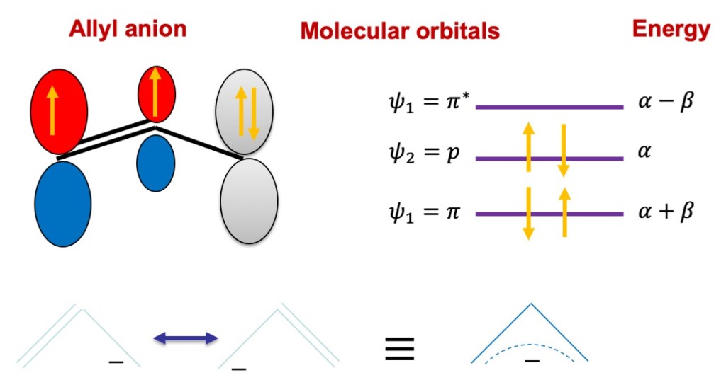
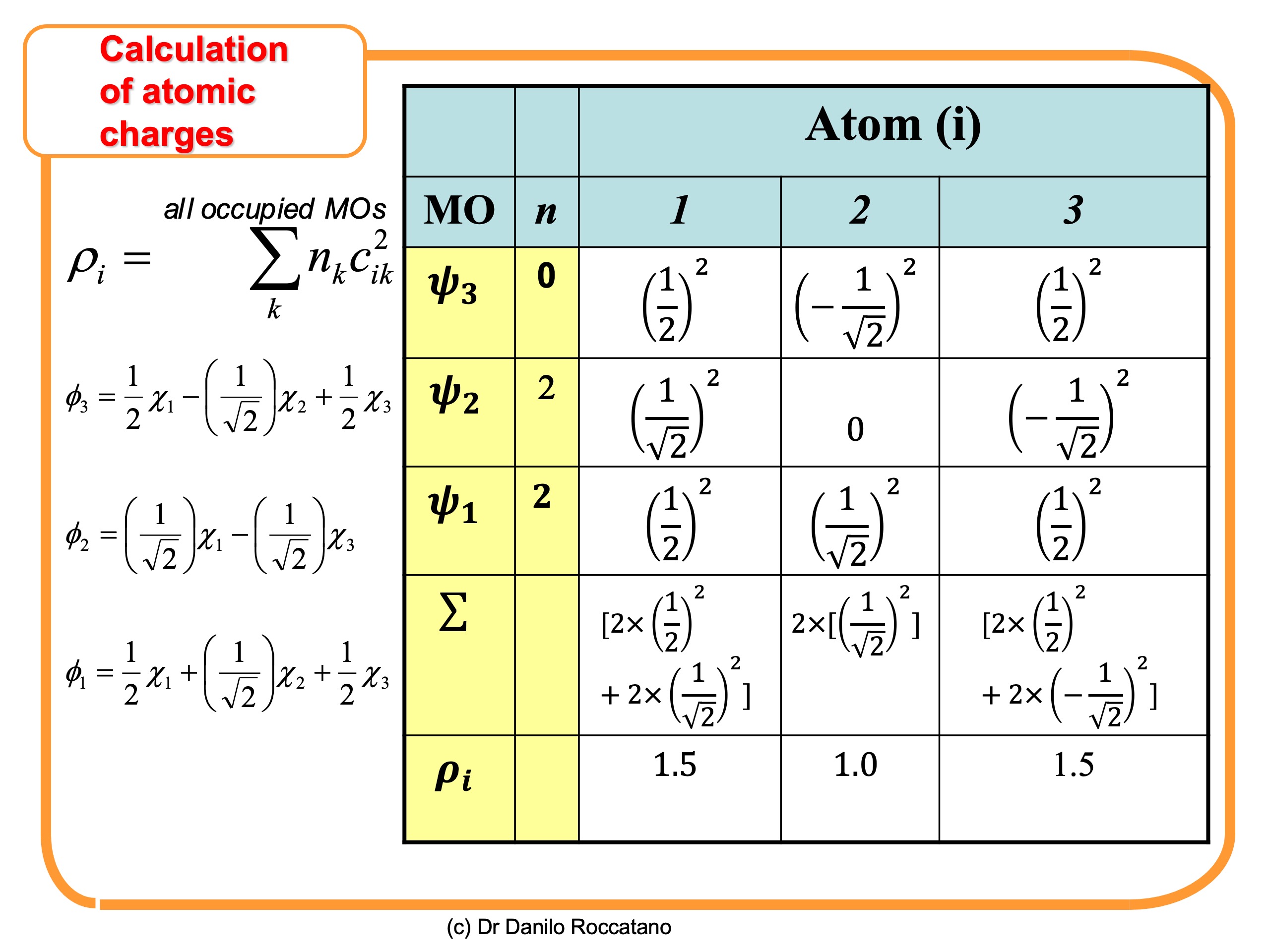
of the allyl radical is reported. The result shows an equal contribution of 0.707 for both bonds.

The total bond order is obtained by adding the sigma bond (1) to P_{ij} 
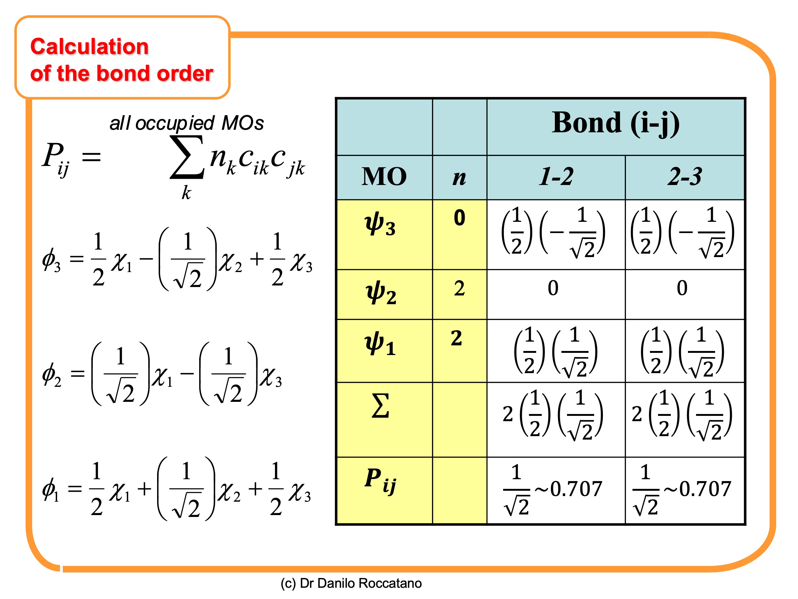
as shown in the examples reported in the figure below.

For hydrocarbons, there is a correlation between bond order and bond lenght that can be used to make an approximate prediction of bond lenght variations. C.A.Coulson in article of 1939 has proposed the following formula that can be used to estimate the effect of the bond order on the length variation of a single bond

$$R=s-\frac{s-d}{1+\frac{k(1-p)}{p}}$$

where s is the average single bond length taken equal to 1.54 A for C-C, d, the double bond length equla to 1.337 A, p the bond order, and k an adjustable parameter. For the example given before, gor p=0.707 and k=0.795, the value of R is

$$R=1.54-\frac{1.54-1.337-d}{1+\frac{0.795(1-0.707)}{0.707}}=1.54-0.153=1.387 \AA$$

CHEMICAL REACTIVITY INDECES

CALCULATION OF THE FREE VALENCE

Finally, the free valence is defined as the difference between the maximum possible bond order and the actual tital bond order. It is defined as

F_i=\sqrt{3}-\sum_k^{\textrm{all occupied MOs}} n_k c_{ik} c_{jk} = 1.732 -\sum_k^{\textrm{all occupied MOs}} n_k c_{ik} c_{jk}

Slide43

UNDER CONSTRUCTION

If you have found interesting and useful my article, do not forget to press “Like it” and subscribe for updates on new ones!

REFERENCES

  1. J. P. Lowe. Quantum Chemistry. 1993, Academic Press. 
  2. F.A. Carroll. Structure and Mechanism,1998, BROOKS/COLE Publishing Company.

Physical Chemistry: The Simple Hückel Method (Part III)

In the previous article, we have learned how to set up the Hückel determinant for conjugated linear molecules based on the topology of the \pi-
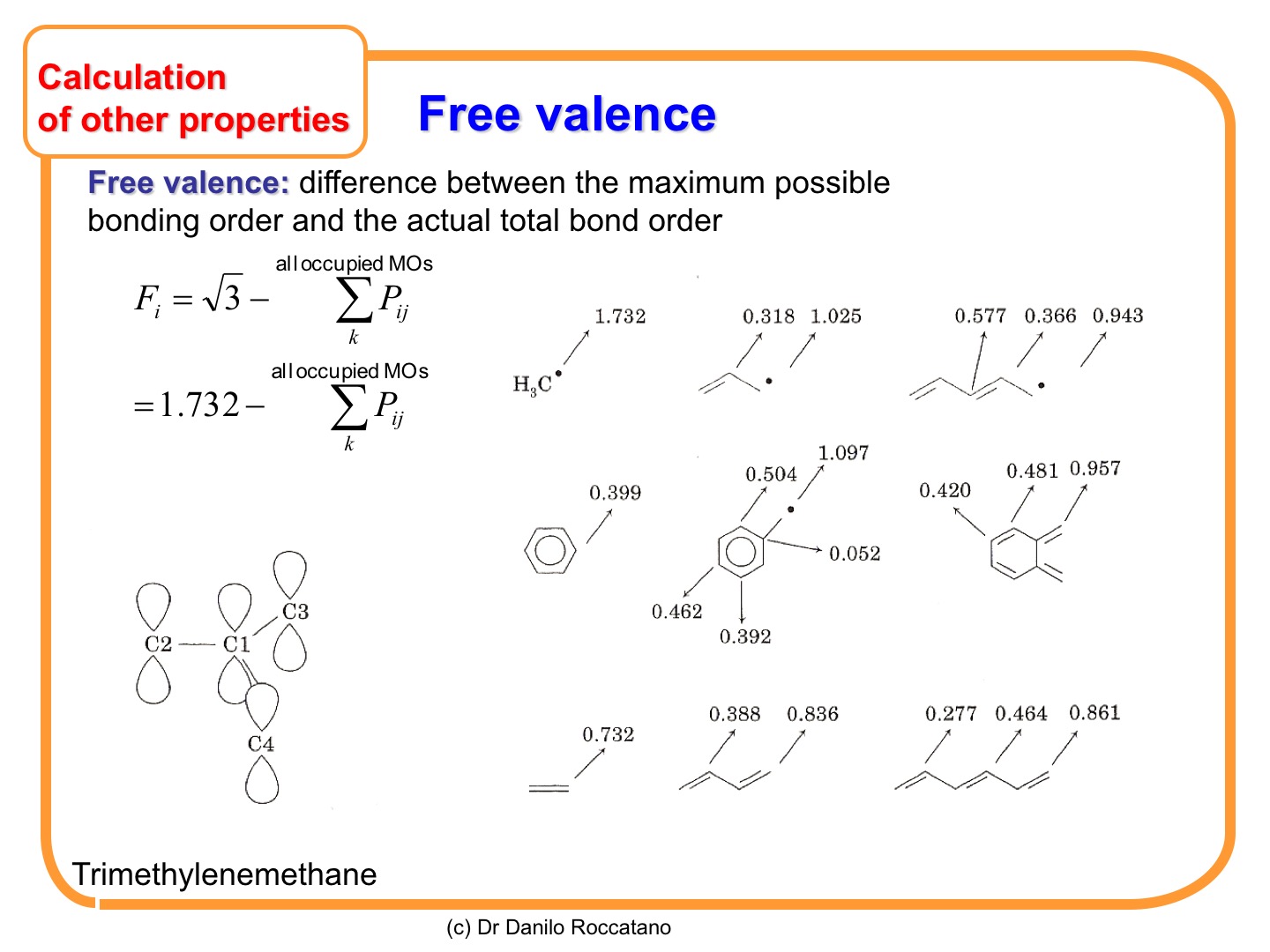
bonds. In this third article, we will apply the method to cyclic molecules and will derive some other useful properties.

Continue reading

Physical Chemistry: The Simple Hückel Method (Part II)

In the previous article, we have learned how to set up the Hückel determinant for an aromatic molecule based on the topology of the pi-bonds. In this second part, we are going to learn how to calculate from the determinantal equation both the eigenvalues and the eigenvectors, corresponding to the orbital energy and orbital functions of the molecular system.

Continue reading

A Practical Introduction to the C Language for Computational Chemistry. Part 2

In the first part of this introduction to C language, we have learnt the basic of the C language by writing simple programs for the calculation of the non-bonded interaction between two particles at variable distances. Some solutions to the first part exercises are reported in the appendix of this article.

In this second tutorial, we will learn how to use arrays data types and how to load them with a set of data read from a file. We will also use these data to perform numerical calculations and write results in output files.

Arrays and Pointers Datatypes

The program that calculate the energy of interaction between two particle doe not take in account the actual position in space of the two particle but only their distance. If we want to study the dynamics of a system composed by multiple atoms in a tridimensional space, it is way more convenient to represent the and calculate their interactions by using the coordinates directly to evaluate the distances.

Continue reading

The Dandelion (Taraxacum Officinalis) and OpenCV

The dandelion’s pallid tube
Astonishes the grass,
And winter instantly becomes
An Infinite Alas —

The tube uplifts a signal Bud
And then a shouting Flower, —
The Proclamation of the Suns
That septulture is o’er.

– Emily Dickinson

The yellow flowers and the delicate and beautiful inflorescence of Dandelion catch the attention of both romantic and curious souls. The aerial consistency of the fine silk decorated seeds that glance to the sunlight as crystalline material became the favorite subject of the inspired photographers and the toy of amused children. Besides the grace of its forms, other interesting and the curious secret is hidden in its phloem fluids. In fact, if you cut one of the stems of the plant, a milky, sticky liquid will flow out of the wound resection. This latex is going to polymerize at 30-35 oC in a few minutes in a yellow-brown quite solid mass. Around the year 1982, I have annotated this observation but I could not find in my later notes further follow-ups study on the topics. It was a casual observation but I didn’t know at that time that this latex is indeed very useful. A variety of the Taraxacum (Taraxacum koksaghyz, Russian Dandelion) was used in Russian and American to produce a replacement of the natural rubber from Brazil during WWII that was in shortage because of the war. Many studies are in progress to exploit the lattice of Taraxacum and  Taraxacum brevicorniculatumas, a convenient replacement for the rubber plant lattice. A recent study has shown the presence of rubber particles in the lattice of these plants in 32% proportion composed prevalently by poly(cis-1,4-isoprene) at >95% purity (www.biomedcentral.com/1471-2091/11/11). The brownish lattice condensate that, as I reported in my note, forms after exposing the latex to the air for several minutes is caused by the presence of the polyphenol oxidase (PPO) enzyme that produces the fast coagulation of the latex by catalysing the oxidation of polyphenols. Genetic engineering the plant makes it possible to reduce the amount of PPO in the latex, making economically competitive use of this resource for latex production.

Continue reading