Cellular automata (CA) is a vast and interesting topic of computer science and mathematics with important applications in many areas of science. They are used to describe deterministic processes involving transitions (i.e. defined by rules) of the state of entities called cells. The game of life (see my previous post) is a famous example of a two-dimensional cellular automaton. However, even simpler cellular automata than the game of Life automata can show peculiar behavior. The famous mathematician Stephan Wolfram has dedicated a lot of time to study such peculiar computational creatures. In A New Kind of New Science, he gives a detailed description of CA of different types. However, my first encounter with CA occurred in the ’80s within the pages of Le Science magazine (the Italian edition of Scientific American). In particular, I was inspired by the amusing A. K. Dewdney’s Computer Recreations department that every month was a source of very interesting programming ideas. Dewdney described different types of cellular automata from the game of Life to the one-dimensional (1D) ones. In this blog, I am going to present a program written in awk language that simulates 1D CA on a computer terminal.
A 1D CA is composed of a sequence of entities called cells each of them characterized by a state (designed by a number) and a set of rules that change this state in time. The CA is a dynamical system iterative system that changes the state of all the cells at the same time (parallelism) at each iteration step. The simplest CA is characterized by a binary state (0,1, as for the game of Life). However, it is possible to design more complex automaton with more states. At the beginning of a CA interaction (step=0), each CA cell is assigned to an initial state. At each iteration step, the state of each cell is updated by the same set of transition rules (homogeneity) defined by the state of the neighbor cells (locality). In the simplest 1D CA, the two first neighbor cells are considered.
Transition functions. The transitions for this simple model of CA can be classified using a three-bit code system as shown in Figure 1. The three upper square defines a portion of the automaton, and we are interested to follow the transition of the central cell. The two side cells are the first neighbor cells. The single cell below represents the central cell after the transition. Each of the three cells can assume the 8 possible configurations depicted in Figure 1. We can assign 

Figure 1: definition of the 255 rule of the 1D binary CA.
CA classification. We can extend the classification to automata by adding more states but the number of configurations will enormously increase. For example, an automaton defined by three states (0,1,2) can have 


Boundary conditions. Three type of boundary conditions (BC) can be adopted for 1D CA (see Figure 2). In the reflective boundary conditions (RBC), the previous of the first and the subsequent of the last (n) cell of the automaton assume respectively the same state of the two considered cells. While in the Constant Boundary conditions (CBC) the two boundary cells of the automaton are keep to a constant state. Finally, in the Periodic Boundary Conditions (PBC), the extreme cells of the automaton are connected forming a ring.

Figure 2: Type of boundary conditions for 1D CA.
A 1D CA implementation in AWK language
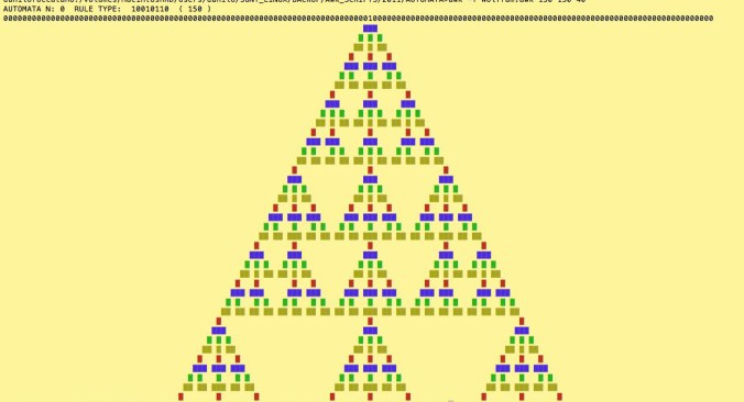
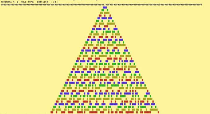
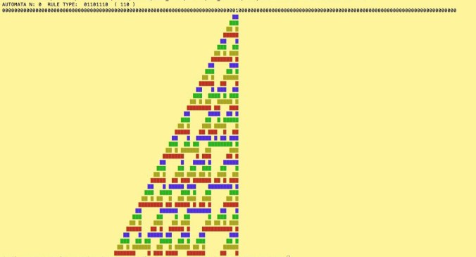
The awk program reported in the appendix implements the 1D CA described in the previous paragraph. The evolution of the CA is represented by printing on the terminal a line at each generation where only the cells with value 1 are shown. For a better identification of the different generation, the program print in 7 different colors the different generation lines.
In the following figures, examples of outputs for some of the rules are reported. For a discussion of these results, the reader can refer to the reported literature.


Bibliography
- S. Wolfram. A New Kind of Science.
- Helene Vivien. An Introduction to CELLULAR AUTOMATA.
- A.K. Dewdney. The armchair Universe. WH. Freeman Company, 1988.
- M. Schroeder. Fractal, Chaos, Power Laws: minutes from an infinite paradise., Dover Ed., 1991.
APPENDIX
Usage:
Wolfram.awk code1 code2 ncycles random
#!/usr/local/bin/gawk -f
#======================================================================
#
# NAME: Wolfram.awk
#
#======================================================================
# DESCRIPTION: Calculate mono dimensional automata
#
# USAGE
# Wolfram code1 code2 ncycles random
#
# INPUT:
#
# RULES SPECIFICATION
# The rules is specified with a decimal value from 0-255.
# It is possible to run different rules in sequence by
# specifying the starting and ending values
# ird : starting rule code (0-255)
# erd : end rule code
# TOPOLOGY SPECIFICATIONS
# N: lenght of the automaton
# BC: boundary conditions (not yet implemented)
# 0: reflective
# 1: constant
# 2: periodic
# SIMULATION SPCIFICATIONS
# ncycles: number of cycles
# STARTING CONFIGURATION
# random = 1 : Random generation
# random = 0 : with one cell at value 1 in position (pos)
# pos: position on the sequence for random=0 (1-N)
# OUTPUT:
#======================================================================
# DEVELOPED USING: gawk
# REQU. FUNCTIONS:
#
# get01string(innum, t, retstr, i) {
# This function return the binary representation of a decimal number
# and it was found on internet and written by Tim Sherwood
#
#======================================================================
# Author: Danilo Roccatano
# Version: 0.2
# Copyright (C): 2016 Danilo Roccatano
# Created: 2016-07-07 20:33
#======================================================================
BEGIN {
#
# INPUT SECTION
#
if (ARGC <3) {
print "SYNTAX: Wolfram code1 code2 ncycles "
exit -1
}
ird= ARGV[1]
erd= ARGV[2]
ncycles = 10
ncycles= ARGV[3]
BC=2 # set as periodic conditions
#
# Calculate the terminal size
#
TermSize()
#
# Take the lattice size from the number of column in the current
# terminal
#
N=cols
random = 0
pos = int(N/2)
#
# Uncomment the following line to have
# if you want to override the default values
# N= ARGV[3]
# random= ARGV[4]
# pos= ARGV[5]
# BC= ARGV[6]
nrl = erd-ird
for (i=0;i<=nrl;i++) {
lrule[i]=ird
ird++
}
#
# Define the automata transition rules and symbols
#
defrule()
#
# === PROGRAM START
# Loop on the rules
#
for (rl = 0; rl <= nrl;rl++) {
rd = lrule[rl]
tt=get01string( rd)
if (length(tt) <8) {
tt = "00000000" tt
rb = substr(tt,length(tt)-7,8)
} else {
rb = tt
}
print "AUTOMATA N:",rl," RULE TYPE: ",rb," (",rd,")"
#
# Generate the starting configuration
# random == 1 : Cells are randomly set to 1 or 0.
# random == 0 : Central cell set to 1 the rest to zero.
#
atms=GenConf(random,BC,N, atm)
#
# Time evolution of the automata
#
tatm=""
print substr(atms,2,length(atms)-2)
for (k=1;k<=ncycles;k++) {
#
# Loop on the automata
#
for (i=2;i<=N+1;i++) {
ncel=substr(atms,i-1,3)
#
# Apply the transition on the triplet ncel
#
for (j=0;j<8;j++) {
if (crul[j] ~ ncel) {
vv=substr(rb,j+1,1)
grap=grap sym[vv]
tatm=tatm vv
}
}
}
#
# Apply the BC conditions to the string tatm
# by adding to the offset cell at the beginning (0) and
# to the to the end (N) values accordingly to the BC variable setup as follows
#
# =0: reflective: add the values of the first and to the last cell of the current lattice, respectively.
# =1: constant: add the value in ccel variable
# =2: periodic: add the values of the last and the first cell of the current lattice, respectively.
#
if (BC == 0) {
tatm = substr(tatm,1,1) tatm substr(tatm,length(tatm),1)
}
else if (BC ==1) {
tatm = ccel tatm ccel
} else {
tatm = substr(tatm,length(tatm),1) tatm substr(tatm,1,1)
}
atms=tatm
tatm=""
#
# Print the new generation line in color with period 4
#
if (k%7 == 0) color(grap,"red")
if (k%7 == 1) color(grap,"blue")
if (k%7 == 2) color(grap,"green")
if (k%7 == 3) color(grap,"yellow")
if (k%7 == 4) color(grap,"purple")
if (k%7 == 5) color(grap,"cyan")
if (k%7 == 6) color(grap,"lightgray")
printf "\n"
grap=""
}
} # end cycle on the list of rules
}
function color(s,co) {
switch (co) {
case "red":
printf "\033[1;91m"s"\033[0m"
break
case "green":
printf "\033[1;32m"s"\033[0m"
break
case "blue":
printf "\033[1;34m"s"\033[0m"
break
case "yellow":
printf "\033[01;33m"s"\033[0m"
break
case "purple":
printf "\033[01;35m"s"\033[0m"
break
case "cyan":
printf "\033[01;36m"s"\033[0m"
break
case "lightgray":
printf "\033[01;37m"s"\033[0m"
}
}
func get01string(innum, t, retstr, i) {
# Return the binary representation of a decimal number
# by Tim Sherwood
retstr = "";
t=innum;
while( t )
{
if ( t%2==0 ) {
retstr = "0" retstr;
} else {
retstr = "1" retstr;
}
t = int(t/2);
}
return retstr;
}
func defrule() {
crul[0]="111"
crul[1]="110"
crul[2]="101"
crul[3]="100"
crul[4]="011"
crul[5]="010"
crul[6]="001"
crul[7]="000"
sym["0"]=" "
sym["1"]="â"
}
function TermSize() {
cmd="tput lines"
cmd | getline lines
lines=lines-2
cmd="tput cols"
cmd | getline cols
}
function GenConf(random,BC,N, atm,atms)
{
#
# Generate the starting configuration
# random == 1 : Cells are randomly set to 1 or 0.
# random == 0 : Central cell set to 1 the rest to zero.
#
if (random == 1) {
srand()
for (i=1;i<N+1;i++) {
a=rand()
val =1
vals = "1"
if (a<0.5) {
val = 0
vals = "0"
}
atm[i]=val
atms = atms vals
if (i==1) first = vals
}
} else {
atms=""
for (i=1;i<N+1;i++) {
vals = "0"
val=0
if (i== pos) { vals = "1";val=1}
atms = atms vals
atm[i]=val
if (i==1) first = vals
}
}
#
# Assign the last cell the same value of the first one
#
tatm=atms
if (BC == 0) {
tatm = substr(tatm,1,1) tatm substr(tatm,length(tatm),1)
}
else if (BC ==1) {
tatm = ccel tatm ccel
} else {
tatm = substr(tatm,length(tatm),1) tatm substr(tatm,1,1)
}
atms=tatm
return atms
}


Pingback: Programming in Awk Language. LiStaLiA: Little Statistics Library in Awk. Part II |