My heart leaps up when I behold
A rainbow in the sky:
So was it when my life began;
So is it now I am a man;
So be it when I shall grow old,
Or let me die!
The Child is father of the Man;
And I could wish my days to be
Bound each to each by natural piety.William Wordsworth, March 26, 1802
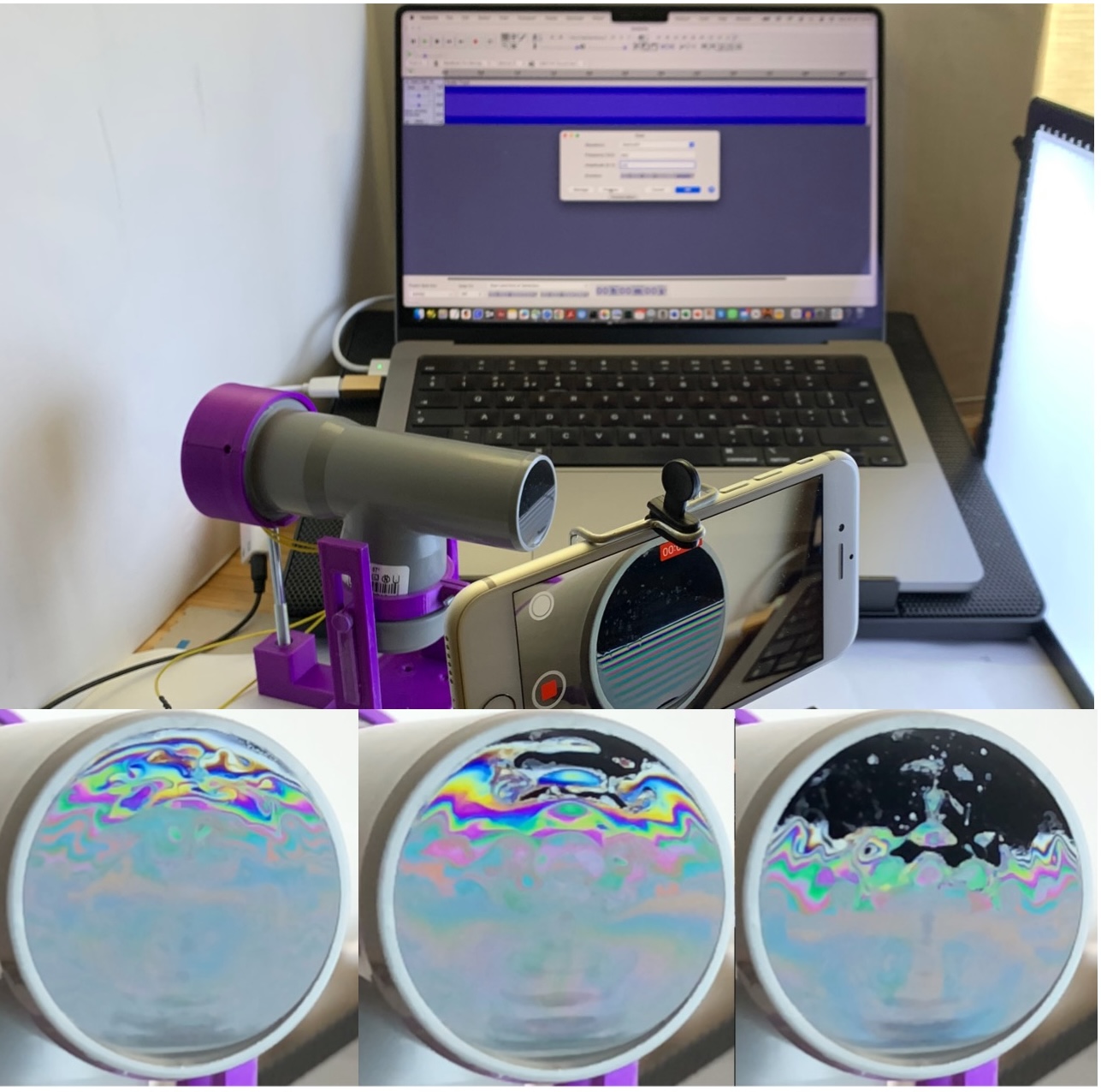
I couldn’t resist citing the beautiful poetry by Wordsworth about the rainbow to introduce my new Instructable, ‘Explore the Physics of Soap Films with the SoapFilmScope.’ I got the idea for this project by reading an article by Gaulon et al. [1]. The authors describe in detail the use of soap film as an educational aid to explore interesting effects in the fluid dynamics of this system. In particular, they examine the impact of acoustic waves on the unique optical properties of the film. In this Instructable, we have designed a device called the SoapFilmScope to perform these experiments. This tutorial will guide you through the process of creating this device, showcasing the mesmerizing interaction between sound waves and liquid membranes. The SoapFilmScope offers an engaging way to explore the physics of acoustics, light interference, and fluid dynamics.
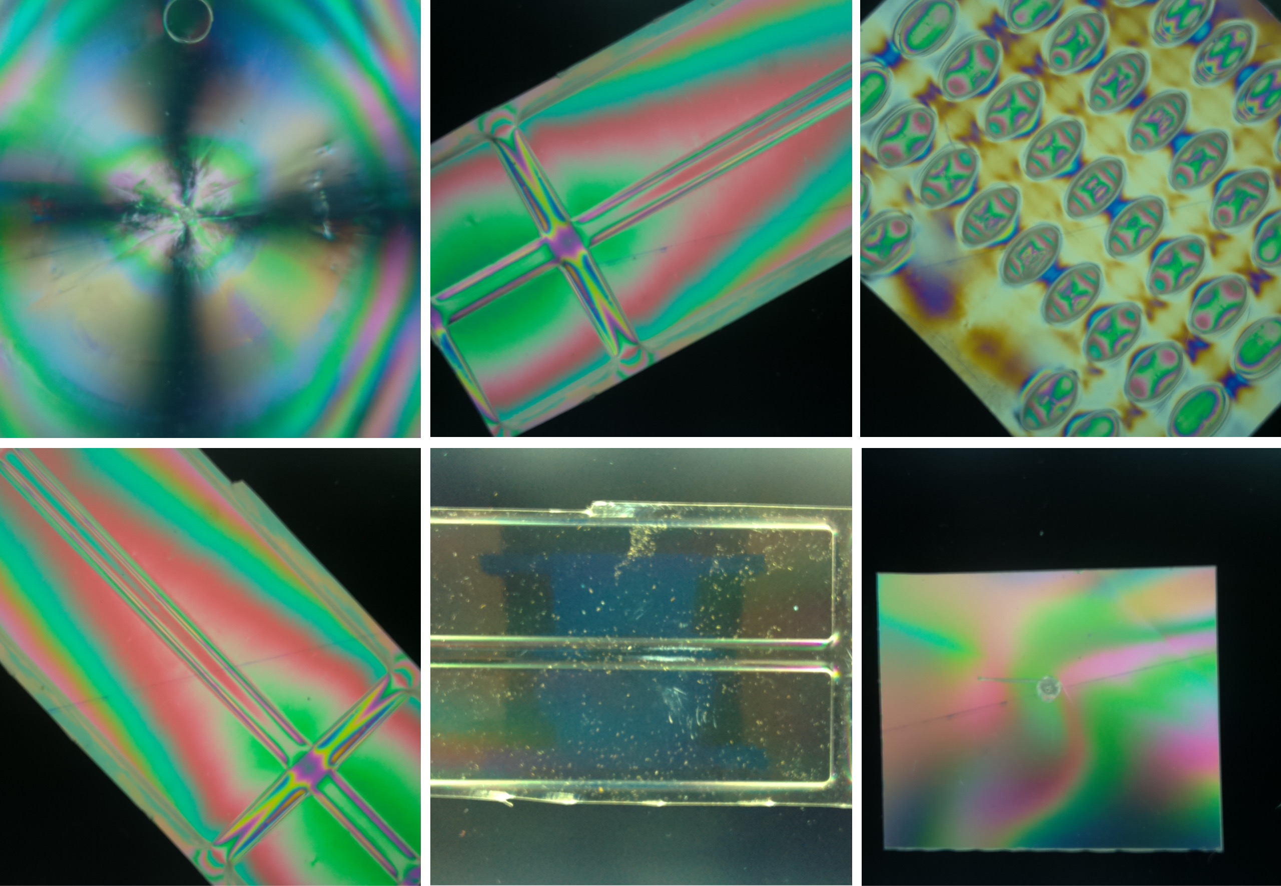
When a sound wave travels through the tube and vibrates the soap film, it creates dynamic patterns through several fascinating mechanisms:
The device consists of a vertical soap film delicately suspended at the end of a tube obtained from a PVC T-shaped fitting that you can get from any DIY store. By attaching a small inexpensive speaker to it, you can let the film dance to the rhythm of the music.