In college, before video games, we would amuse our- selves by posing programming exercises. One of the favorites was to write the shortest self-reproducing pro- gram. Since this is an exercise divorced from reality, the usual vehicle was FORTRAN. Actually, FORTRAN was the language of choice for the same reason that three-legged races are popular.
Ken Thompson, Communications of the ACM. 27 (8), 761–763, 1984.
In December of last year, I celebrated the 30th anniversary of my Laurea in Chemistry dissertation. The starting of my thesis dissertation also signed my acquaintance to one of the grannies of the scientific programming languages, FORTRAN. Since then, I have used and (continue to) this language for my research activity by writing several thousands of lines of code. Therefore, I want to share some of my modest programming achievements using this language.
I will concisely introduce this captivating programming language in a series of articles. This is a primer on a programming language with much more to offer, especially in the new versions starting from the FORTRAN 90. Readers interested in deepening their knowledge in FORTRAN can find online many excellent tutorials and discussion groups, as well as plenty of excellent textbooks that have been written.
The FORTRAN language
Fortran (FORmula TRANslation) language was introduced in 1957 and remains the language of choice for most scientific programming. The language was constantly restyled and updated (e.g. Fortran IV, Fortran 77). Recent improvements, recently introduced with the Fortran 90 and 95/2003, include several extensions in more modern languages (e.g. in the C language). Some of the most important features of Fortran 90/95 include recursive subroutines, dynamic storage allocation and pointers, user-defined data structures, modules, and the ability to manipulate entire arrays. Fortran 90 is compatible with Fortran 77 but not the other way around. However, the new Fortran language has evolved in a modern computer language by incorporating constructs from other languages.
Writing and compiling Fortran programs.
Fortran programs can be edited using one of the many text editors available in Unix OS. From Fortran 90, Fortran language has left the traditional fixed format, the legacy of a prehistoric computer era dominated by punched card input devices (http://en.wikipedia.org/wiki/Punched_card),
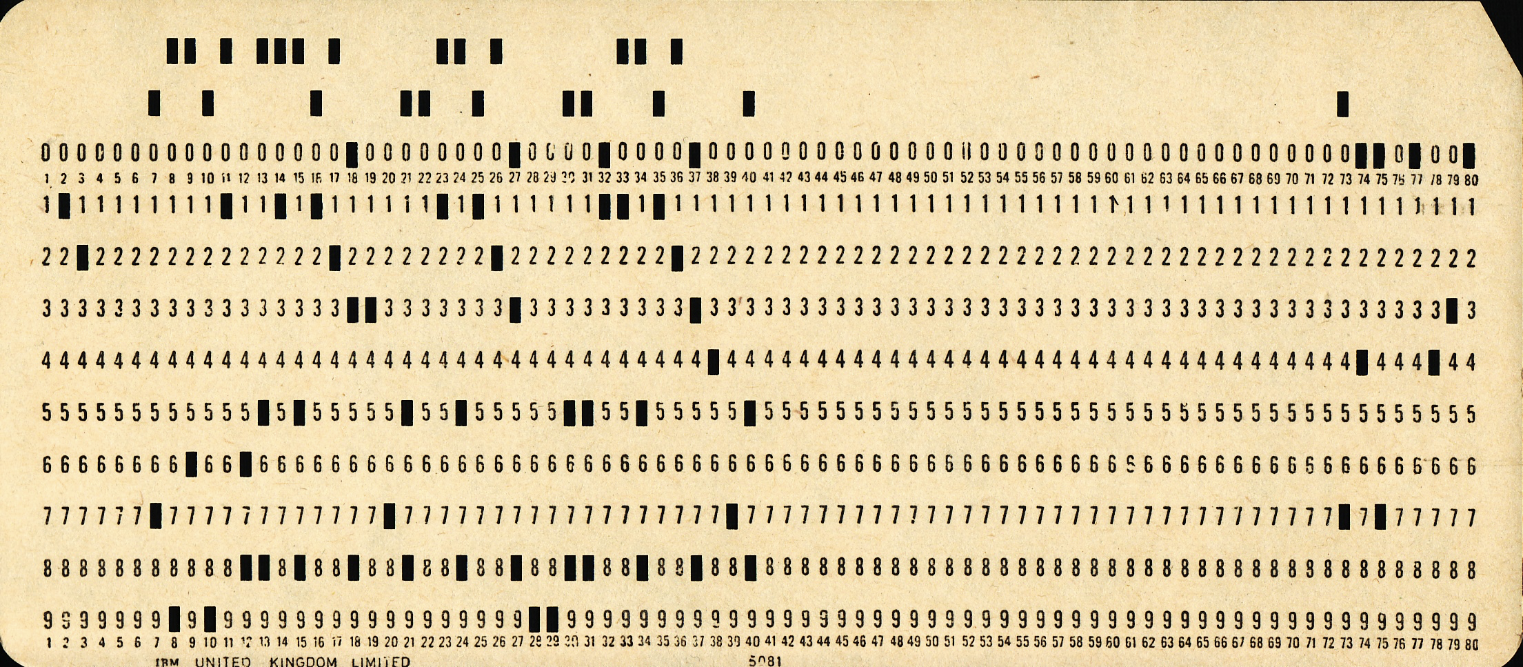
12 PIFRA=(A(JB,37)-A(JB,99))/A(JB,47) PUX 0430
source: wikipedia.
to the more convenient free format. This means you can write the instruction everywhere along each line of the program. Once the program is written (remember to terminate it with the end statement), save it with a root name (e.g. integration) and the file extension .f (e.g. integration.f). The next step is the compilation of the program, namely the transformation of the human-readable source code into the computer language binary code. This can be performed with the following command:
gfortran integration.f –o integration
The program is then executed using the command:
./integration
STRUCTURE OF A FORTRAN PROGRAM
The first statement of the program (PROGRAM) defines the program’s name; the last statement must have a corresponding END program statement. Comments begin with a ! and can be included anywhere in the program. Statements are written on lines which may contain up to 132 characters.
DATA TYPES STRUCTURES
Numerical and alphanumerical data are assigned to a specific memory location of the computer using variables. A variable is defined with a name and a type. The names of all variables must be between 1 and 31 alphanumeric characters, of which the first must be a letter, and the last must not be an underscore. The types of all variables are declared at the beginning of the program. There are 5 build-in variable types:
– integer Integers
– real Floating point numbers
– complex Complex numbers
– logical Boolean values
– character Strings and characters
In many Fortran 77 one can see statements like
IMPLICIT REAL*8(a-h,o-z)
meaning that all variables beginning with any of the above letters are, by default, floating numbers. However, such usage makes it hard to spot eventual errors due to misspelling variable names. With IMPLICIT NONE you have to declare all variables and therefore detect possible errors already while compiling; hence, it is strongly recommended.
The syntax for a variable declaration is:
type [[,attribute]… ::] entity-list
Examples
integer :: a
real :: b
logical :: flag
character :: ch
character(len=80) :: line
Floating point numbers are assigned as REAL (REAL*8 or REAL(8) for double precision).
Arrays and matrices
An array is declared in the declaration section using the dimension attribute.
Examples
real(8) :: fe(6)               ! Array with 6 elements
real(8), dimension(20,20) :: K ! Matrix 20x20 elements
real(8) :: fe(6)               ! Array with 6 elements
real(8), dimension(20,20) :: K ! Matrix 20x20 elements
The default value of the lower bound of an array is 1. The last statement is an example of a two-dimensional array.
Allocate statement and mathematical operations on arrays
One of the better features of Fortran 90 is dynamic storage allocation. That is, the size of an array can be changed during the execution of the program. However, the arrays to be allocated must be defined at the beginning of the program. The allocation of the variable is then performed using the command allocate. The following example illustrates how this is done.
Example
! Definition of allocable arrays

real , dimension (:) , allocatable :: f
real , dimension (: ,:), allocatable :: K
allocate (K(20 ,20) )
allocate ( f (20) )
The following code illustrates that when the allocated memory is no longer needed, it can be deallocated using the command deallocate().
Examples
deallocate (K)
deallocate (f)
An important issue when using a dynamically allocatable variable is to make sure the application does not” leak”.” Leaking” is a term used by applications that allocate memory during the execution and never deallocate used memory. If unchecked, the application will use more resources and eventually make the operating system start swapping and perhaps become unstable. Therefore, a rule of thumb is that an allocate statement should always have a corresponding deallocate.
VARIABLE ASSIGNMENT
A logical variable can assume two values, true (1) and false (0).
Example
Logical :: flag
flag = .false.
flag = .true.
The assignment of strings is illustrated in the following example.
character(40) :: firstname
character(40) :: lastname
firstname = “mickey”
lastname = ”mouse”
The first variable, first name, is assigned the text “mickey“. The remaining characters in the string will be padded with spaces. Next, a string is assigned using citation marks,” or apostrophes,’. This can help when using apostrophes or citation marks in strings.
Arrays are assigned values either by explicit indices or the entire array in a single statement. For example, the following code assigned the variable, K, the value 5.0 at position row 5 and column 6.
real(8), dimension(20,20) :: K ! Matrix 20x20 elements
K(5,6)=5.0
If the assignment had been written as
K(5,6)=5.0
the entire array, K, would have been assigned the value 5.0. This is an efficient way of setting the whole array’s initial values.
Explicit values can be assigned to arrays in a single statement using the following assignment.
real(8):: v(5) ! Array with 5 elements
v = (/ 1.0, 2.0, 3.0, 4.0, 5.0 /)
This is equivalent to an assignment using the following statements.
v(1) = 1.0
v(2) = 2.0
v(3) = 3.0
v(4) = 4.0
v(5) = 5.0
The number of elements in the list must be the same as the number of elements in the array variable.
Assignments to specific parts of arrays can be achieved using index notation. The following example illustrates this concept.
program index_notation
implicit none
real :: A(4,4)
real :: B(4)
real :: C(4)
B = A(2,:) ! Assigns B the values of row 2 in A
C = A(:,1) ! Assigns C the values of column 1 in A
stop
end program index_notation
Using index notation, rows or columns can be assigned in single statements, as shown in the following code:
! Assign row 5 in matrix K the values 1,2,3,4,5
K(5,:) = (/ 1.0, 2.0, 3.0, 4.0, 5.0 /)

! Assign the array v the values 5, 4, 3, 2, 1
v = (/ 5.0, 4.0, 3.0, 2.0, 1.0 /)
MATHEMATICAL, LOGICAL AND RELATIONAL OPERATORS
The following arithmetic operators are defined in Fortran:
** : power to
* : multiplication
/ : division
+ : addition
– : subtraction
Parenthesis are used to specify the order of different operators. For example, if no parenthesis are given in an expression, operators are evaluated in the following order:
1. Operations with **
2. Operations with * or /
3. Operations with + or –
Example
Calculation of the area of a circle given its radius
Note in this example we are going to use the statments for performing I/O operation on the screenand keyboard device.
To input the data from the keyboard, we use the command
          print *, "Insert radius:"
          read(*,*) raggio
Th print statment print the message “Insert radius:” followed but the next statment that read a value from the keyboard and assign to the floating point variable raggio.
The statment
write (*,*) mess,area
write on the console screen the message “Area del cerchio :” (assigned to the character variable mess) folllowed by the value of the calculated area.
     program Calc_area_circle

          real pigro, raggio,area
          character mess*20

          mess="Area of the circle: "
          pigro=3.14159265359

          print *, "Insert radius:"
          read(*,*) raggio

          area=pigro*raggio*raggio

          write (*,*) mess,area

      end program
Copy the program in a file named, for example, circle.f.
Compile it using the command
gfortran circle.f -o Circle
run the executable as
./Circle
 Insert radius:
 2.45
 Area of the circle:    18.8574104
Intrinsic Mathematical Functions
Intrinsic mathematical function (IMF) are used as
y=IMF(x)
where x, y are the argumento of the function anf y the return variable. In the following the more common function are listed.
The last two column represent the type of variable expected for the argument and the return value.
| Function | Mathematical operation | Arg. Type | Return Type |
| ABS(x) | absolute value of x | INTEGER/REAL | INTEGER/REAL |
| SQRT(x) | square root of x | REAL | REAL |
| SIN(x) | sine of x | REAL | REAL |
| COS(x) | cosine of x | REAL | REAL |
| TAN(x) | tangent of x | REAL | REAL |
| ASIN(x) | arc sine of x | REAL | REAL |
| ACOS(x) | arc cosine of x | REAL | REAL |
| ATAN(x) | arc tangent of x | REAL | REAL |
| EXP(x) | exponential of x | REAL | REAL |
| LOG(x) | natural logarithm of x | REAL | REAL |
| LOG10(x) | bases 10 logarithm of x | REAL | REAL |
| SRAND(SEED) | Seeding of the random number generator using the integer SEED | INTEGER | – |
| RAND() | Returns a pseudo-random number from a uniform distribution between 0 and 1. | INTEGER | REAL |
Example
Calculate the distance between two points in 3D space
using the formula

PROGRAM distance3d

    !=======================================================
    !
    !     CALCULATE THE DISTANCE BETWEEN TWO POINTS
    !     GIVEN THIR COORDINATES IN A REFERENCE FRAME
    !
    !=======================================================

    REAL :: x(2),y(2),z(2),dist
    CHARACTER (LEN=10) :: mess
    mess='Distance: '

! Input coordinates

    print *, "Insert coordinates as space separated values (x y z) for the "
    print *, "point A:"
    READ (*,*) x(1),y(1),z(1)
    print *, "and point B:"
    READ (*,*) x(2),y(2),z(2)

! Calculate the distance

    dist=SQRT((x(1)-x(2))**2+(y(1)-y(2))**2+(z(1)-z(2))**2)

    WRITE (*,*) mess,dist

END PROGRAM distance3d
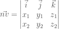
Calculate the magnitute, dot-product and cross-product of two vectors
Given the two vectors defined in 


On the contrary, the cross product results in a vector perpendicular to the plane of the given ones whose components along the cartesian axis $latex (\vec{i}, \vec{j}, \vec{k} ) are given by expanding the determinat
PROGRAM DotandCrossP3D

    !=======================================================
    !
    !     CALCULATE THE CROSS AND DOT PRODUCT OF TWO VECTORS
    !
    ! Roccatano (c) 2015
    !=======================================================

    REAL :: x(3),y(3),z(3),lv(3),dotp,dotpF90
    REAL, dimension(3) :: xv,yv
    REAL :: nv(3)
    CHARACTER (LEN=13) :: mess(4)
    mess(1)='  DOT PRODUCT'
    mess(2)='   COS(THETA)'
    mess(3)='NORMAL VECTOR'
    mess(4)='LENGHT VECTOR'

    ! Input coordinates

    print *, "Insert coordinates as space separated values (x y z) for the "
    print *, "point A:"
    READ (*,*) x(1),y(1),z(1)
    print *, "and point B:"
    READ (*,*) x(2),y(2),z(2)
    xv(1)=x(1)
    xv(2)=y(1)
    xv(3)=z(1)
    yv(1)=x(2)
    yv(2)=y(2)
    yv(3)=z(2)

    ! Calculate vector's lengths

    lv(1)=SQRT(x(1)**2+y(1)**2+z(1)**2)
    lv(2)=SQRT(x(2)**2+y(2)**2+z(2)**2)

    dotp=x(1)*x(2)+y(1)*y(2)+z(1)*z(2)
    dotpf90 = DOT_PRODUCT(XV, YV)
    cost=dotp/(lv(1)*lv(2))

    ! Cross product: normal vector

    NV(1)=y(1)*z(2)-y(2)*z(1)
    NV(2)=z(1)*x(2)-z(2)*x(1)
    NV(3)=x(1)*y(2)-x(2)*y(1)

    lv(3)=SQRT(nv(1)**2+nv(2)**2+nv(3)**2)

    WRITE (*,*) mess(4),"  1:",lv(1)
    WRITE (*,*) mess(4),"  2:",lv(2)

    WRITE (*,*) mess(1),"   :",dotp
    WRITE (*,*) mess(1),"f90:",dotpf90
    WRITE (*,*) mess(2),"   :",cost
    WRITE (*,*) mess(3),"   :",NV(1),NV(2),NV(3)
    WRITE (*,*) mess(4)," NV:",lv(3)
    WRITE (*,*) mess(4),"f90:",norm2(nv)

END PROGRAM DotandCrossP3D
COMMAND FOR CONVERSION OPERATIONS
| Function | Mathematical operation | Arg. Type | Return Type |
| INT(x) | integer part x | INTEGER/REAL | INTEGER |
| NINT(x) | nearest integer to x | REAL | INTEGER |
| FLOOR(x) | greatest integer less than or equal to x | REAL | INTEGER |
| FRACTION(x) | the fractional part of x | REAL | REAL |
| REAL(x) | convert x to | REAL | INTEGER/REAL |
| MAX(x1, x2, …, xn) | maximum of x1, x2, … xn | INTEGER/REAL | INTEGER/REAL |
| MIN(x1, x2, …, xn) | minimum of x1, x2, … xn | INTEGER/REAL | INTEGER/REAL |
| MOD(x,y) | remainder x – INT(x/y)*y | INTEGER/REAL | INTEGER/REAL |
Example
A Random Number generator
Generate a random number using the linear congruential generator. This is the most straightforward implementation of a pseudo-random number generator. The program has been adapted from the RANF routine given in the book by Allen and Tildesley [1]. Note this program is only for didactic application as the quality of the generated a random number depending by the internal representation of the variable type and the set of the (l,c,m) parameter used.
PROGRAM RandomNumbers

    !
    !  CALCULATE A (PSEUDO)RANDOM NUMBER FROM A UNIFORM DISTRIBUTION
    !  IN THE RANGE 0 TO 1.

    INTEGER, PARAMETER :: l = 1029
    INTEGER, PARAMETER :: c = 221591
    INTEGER, PARAMETER :: m = 1048576
    INTEGER :: seed

    print *,"Provide an integer as a seed for starting the generator:"
    READ (5,*) seed

    seed = MOD ( seed * l + c, m )
    ranf = ABS(REAL ( seed ) / m)
    print *,ranf

END PROGRAM  RandomNumbers
CHARACTER STRING OPERATIONS
| Function | String operation | Arg. Type | Return Type |
| LEN(A) | Lenght of string A | CHARACTER | INTEGER |
| TRIM(A) | Remove the black characters in A | CHARACTER | CHARACTER |
| INDEX(A,S) | Return the postion of the string S in A | CHARACTER | INTEGER |
Example
Strings Manipulation
PROGRAM StringManip

    !=======================================================
    !
    !     SOME EXAMPLES OF STRING OPRATION IN FORTRAN
    !
    ! Roccatano (c) 2023
    !=======================================================

    CHARACTER(len=15) :: filename1,filename2

    INTEGER :: length, pos

    filename1  = 'pippo.dat'

    length = LEN(TRIM(filename1))

    print *, "The string ",filename1," contains ",length," characters."

    pos = INDEX(filename1,'po')

    print *, "The po in ",filename1,"is at position:",pos

    filename2  = 'archimede.dat   '

    ! Remove blanks characters and then calculate the lenght

    length = LEN(TRIM(filename2))

    print *, "The second string ",filename2," contains ",length," characters."

    pos = INDEX(filename2,'ch')

    print *, "The ch in ",filename2,"is at position:",pos

    ! Extract the characters from 1 to 5 in filename2 and concatenates (//)
    ! to the charcters 1-5 in the filename1

    print *, "Merging the two strings we obtain the word ",filename2(1:5)//filename1(1:5)

END PROGRAM StringManip


 The string pippo.dat       contains            9  characters.
 The po in pippo.dat      is at position:           4
 The second string archimede.dat   contains           13  characters.
 The ch in archimede.dat  is at position:           3
 Merging the two strings we obtain the word archipippo
REFERENCES
- Allen, M.P. and Tildesley, D.J., 1987. Computer simulation of liquids. Oxford university press

