"… I seem […] only like a boy playing on the sea-shore, and diverting myself in now and then finding a smoother pebble or a prettier shell than ordinary, whilst the great ocean of truth lay all undiscovered before me". – Isaac Newton.
Understanding the Discrete Fourier Transform in Signal Analysis
In previous posts on this blog I have already introduced the Fourier series and the Fourier transform, following their historical development from Joseph Fourier’s original work on heat conduction to their modern role in physics, engineering, and signal analysis. Rather than repeating that material here, I will take it as a starting point.
When we look at a signal — a sound wave, a vibration, or even a curve drawn by hand — we usually perceive it as a function of time or space. However, very often the most relevant information is not immediately visible in this representation. It is hidden in the frequencies that compose the signal, and in how strongly each of them contributes.
This is precisely the idea behind the Discrete Fourier Transform (DFT): to decompose a discrete signal into a finite sum of harmonic components, each characterized by an amplitude and a phase. Conceptually, the DFT is not a new theory, but a practical bridge between the continuous Fourier framework and the realities of digital data, measurements, and numerical simulations.
Rather than starting from abstract formulas, in this post I adopt a visual and experimental approach. The discussion is supported by an interactive program that allows one to draw an arbitrary signal and explore its harmonic content, and by a practical electronics project where Fourier analysis is applied to real sound and noise signals.
The Mathematicsof the DFT
Given a discrete signal sampled at points, the program computes the Fourier coefficients
Each harmonic j contributes:
an amplitude
and a phase
The reconstructed signal is simply the sum of these harmonic contributions. What matters here is not the formula itself, but the idea: any sufficiently smooth signal can be built from sines and cosines.
Complex form of the DFT
In practice it is often more convenient to combine the sine and cosine terms into a single complex expression. The DFT can be written as
and the original signal can be reconstructed through the inverse transform
In this formulation the Fourier coefficient already contains both amplitude and phase information.
The magnitude gives the strength of the harmonic k, while the argument of the complex number provides its phase.
Computational cost
A direct implementation of the DFT requires evaluating N sums, each containing N terms. The total computational cost therefore, scales as operations. For small signals, this is perfectly acceptable, but for large datasets, the cost quickly becomes prohibitive. For example, analysing a signal with samples using the naive DFT would require on the order of arithmetic operations.
The Fast Fourier Transform (FFT)
A major breakthrough came in 1965 when James W. Cooley and John W. Tukey published what is now known as the Fast Fourier Transform (FFT) algorithm.
The key idea is to exploit symmetries in the exponential factor
and recursively split the transform into smaller pieces.
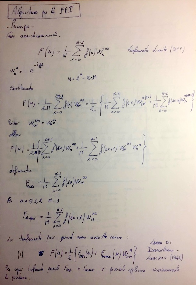
If N is even, the signal can be separated into even and odd indexed samples:
The DFT can then be rewritten as
where the two terms are themselves DFTs of length
By applying this decomposition repeatedly, the original problem of size N is reduced to many smaller transforms of size 2. This divide-and-conquer strategy reduces the computational cost dramatically. Instead of operations, the FFT requires only operations. For large datasets the difference is enormous: what would take hours with a direct DFT can often be computed in milliseconds using the FFT.
The first page shows the derivation of the FFT by splitting the discrete Fourier transform into even and odd indexed samples.This recursive decomposition reduces the original transform of size N into two transforms of size N/2.
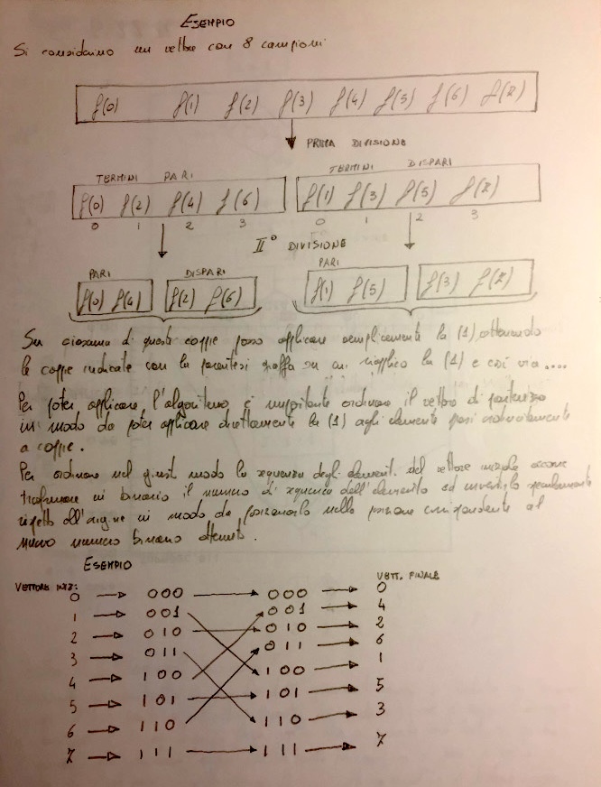
The second part illustrates the bit-reversal permutation used in many radix-2 FFT implementations. Each array index is written in binary form and the order of the bits is reversed to determine the new position of the data.
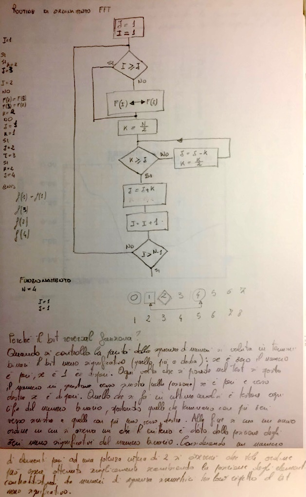
The flowchart describes an algorithm for computing this permutation efficiently before the butterfly stages of the FFT.
The FFT is one of the most important numerical algorithms ever discovered. It is used in an astonishing range of applications, including:
signal processing
image compression
spectroscopy
radar and medical imaging
molecular dynamics simulations
astronomy
In fact, many modern technologies—from digital audio to MRI scanners—rely on the FFT to analyse signals efficiently.
From Drawing a Curve to Harmonic Analysis
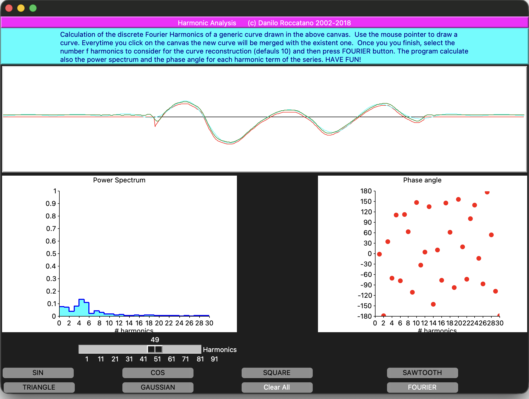
Imagine drawing an arbitrary curve with your mouse on a canvas. The DFT analysis allows us to ask a precise question: Which harmonics are needed to reconstruct this curve, and how important is each one?
In the appendix to this post you will find a Tcl/Tk program that does exactly this:
You draw a signal directly on a canvas (the program also gives the possibility to plot automatically standard signal curves such as the sin, cos, square, triangle, sawtooth, and Gaussian).
The program samples it into a discrete array
A Discrete Fourier Transform is computed explicitly
The signal is reconstructed using a finite number of harmonics
The power spectrum and phase angles are displayed
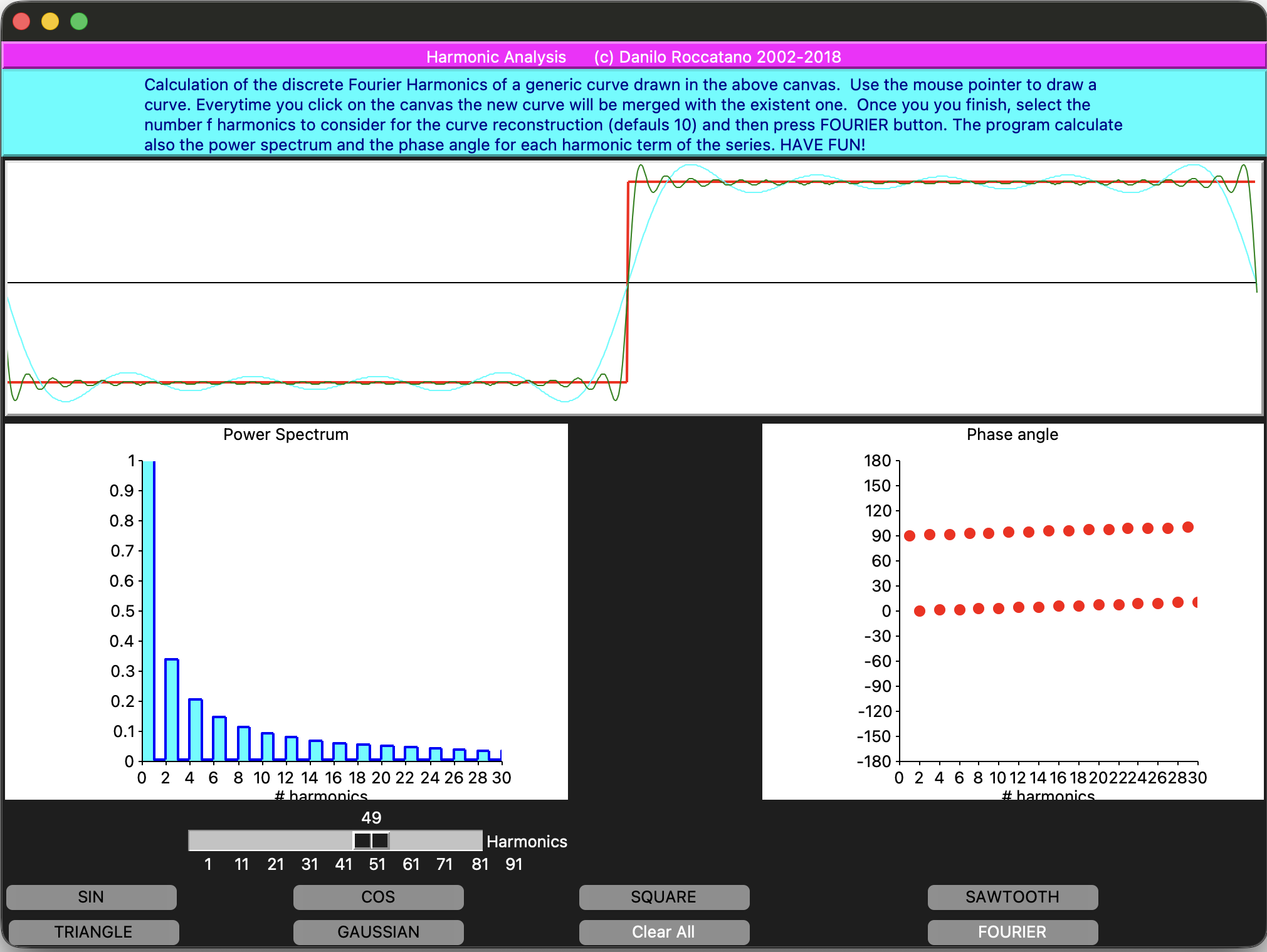
In the figure below, you can see an example of DFT for the square/step signal. You see how adding harmonics improves the reconstruction.
Using the mouse, you can also draw a function on the upper canvas, calculate numerically the Fourier coefficients, and plot a number of terms of your choice from the discrete Fourier series.
The program also plots two key quantities:
The Power Spectrum that shows how much each harmonic contributes to the signal.
The Phase Spectrum that tells us how each harmonic is shifted in time (or space).
These two plots together fully characterize the signal in frequency space.
Fourier analysis is widely used in various scientific and engineering fields. For example in
audio signal processing
vibration analysis
optics
and noise characterization
From Software to Hardware: Exploring Sound and Noise
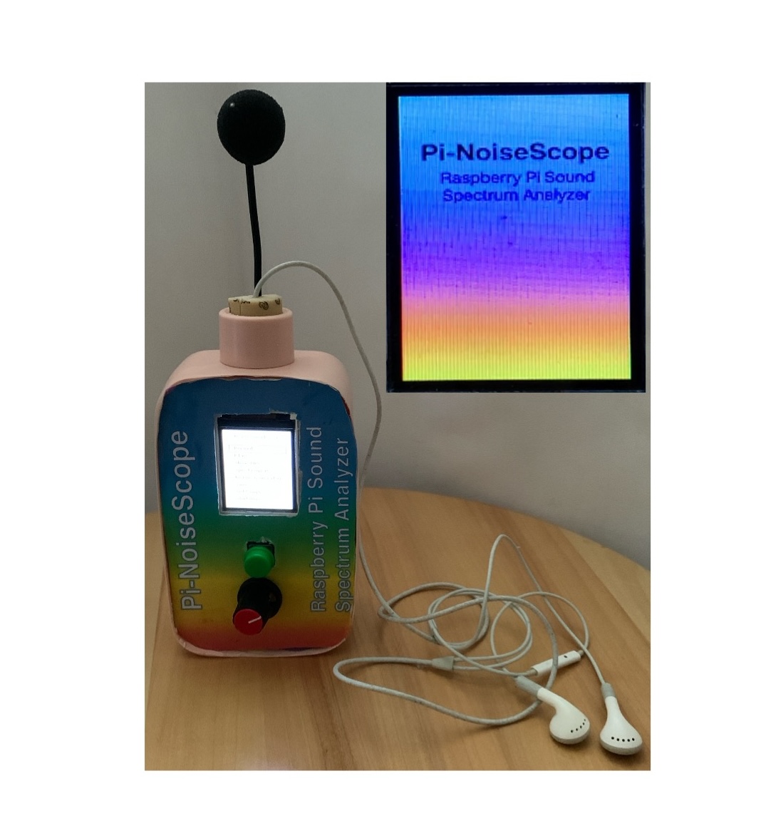
In my recent Instructables projects, I’ve used the Fast Fourier Transform (FFT) to analyse the spectra of sound samples taken with a Raspberry Pi-based device. The project called
In the project, I have build a Sound Analyzer and Generator using a Raspberry Pi (see figure above). This small device, the Pi-NoiseScope, can:
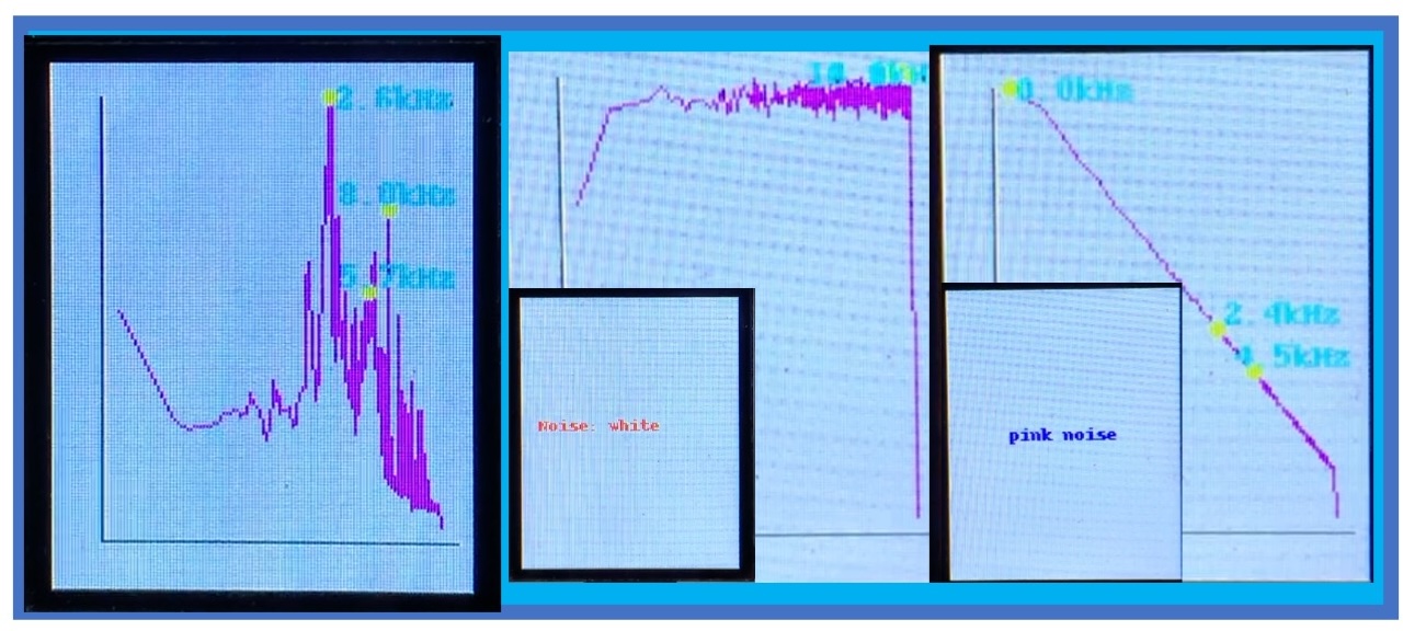
Record ambient sounds and show their frequency spectra
Generate artificial noises of different “colors” (white, pink, brown, blue, violet, etc.)
Fourier analysis reveals the spectral fingerprint of sounds
Display real-time information on a small TFT screen
It lets you explore the beautiful world of sound — revealing that even noise, often thought of as random, hides structure and harmony.
This Tcl/Tk programme serves a similar pedagogical purpose but begins with a software-generated or drawn function before progressing to microphones ADCs and hardware limitations.
Appendix I
Interactive Discrete Fourier Transform Program
Below, you will find the complete source code in Awk and Tcl/Tk programming languages used to perform the harmonic analysis.
It allows you to:
draw arbitrary signals
choose the number of harmonics
visualize reconstruction, power spectrum, and phase
If you enjoy experimenting, try drawing:
a square wave
a triangle
noisy curves
smooth periodic functions
and watch how the frequency content changes.
Have fun exploring the frequency domain!
A program in Awk language to calculate the DFT.
This program read a file containing a list of values representing a function or a signal or a generic set of data to analyze using the harmonical analysis. Then it calculates the Fourier coefficients and finally reconstructs the Fourier series using a given number of terms (n).
#==========================================================
#
# NAME: dft.awk
#
#==========================================================
# DESCRIPTION: Calculate the fourier series of a signal
# INPUT: The program read a two column file containing the
#        signal to elaborate
# OUTPUT: The output contain the reconstructed signal
#         using the first n Fourier components.
#==========================================================
# DEVELOPED USING: gawk
# FUNCTIONS:
# ReadData()    : read a two column data file from stdin
# CalculateDFT(): Calculate the DFT.
# Reconstruct() : Reconstruct/filter the signal using the
#       first n components of the DFT, and print on the
#       stdout thereconstructed signal.
#==========================================================
# Author: Danilo Roccatano
# Version: 1.0
# Copyright (C): 2016 Danilo Roccatano
#==========================================================
#
#

function ReadData() {
#
# Read data from standard input
#
    np=0
    while (getline > 0 ) {
        if (NF >0) {
            P[np]=$2
            np++
        }
    }
    np--
}

function CalculateDFT() {
#
# Perfrom the discrete fourier transform of the data
#
    PI=4*atan2(1,1)
    for (j=1;j<=n;j++) {
        A[j]=0
        B[j]=0
        for (i=0;i<=np-1;i++) {
            x=2*PI*i*j/np
            A[j]+=P[i]*cos(x)
            B[j]+=P[i]*sin(x)
        }
        A[j]/=(np/2)
        B[j]/=(np/2)
    }
}
function CalcA0(){
#
# Calculate the average value of A0
#
    A0=0
    for (i=0;i<=np;i++) {
        A0+=P[i]
    }
    A0=A0/np
}
function Reconstruct() {
    for (i=0;i<=np;i++){
        M[i]=0
        for (j=1;j<=np;j++) {
            F=2*PI*j*i/np
            M[i]=M[i]+A[j]*cos(F)+B[j]*sin(F)
        }
        print i,M[i]+A0
    }
}
BEGIN {

#
# n:= number of armonics to consider
#
n=30
    ReadData()
    CalcA0()

    CalculateDFT()
#
# Reconstruct the signal using n harmonics
#
    Reconstruct()

}
The interactive graphical program in Tcl/Tk language
A program in Tcl/Tk language for the harmonic analysis of a drawn signal This program was inspired by a similar program in BASIC language in a book that I read many years ago [1]. Using the mouse, you can draw a function on the upper canvas, calculate numerically the Fourier coefficients, and plot a number of terms of your choice from the discrete Fourier series.
#! /bin/sh
# the next line restarts using wish \
exec wish "$0" "$@"

###################################################################
#     FOURIER ANALYSIS OF REGULAR AND IRREGULAR FUNCTIONS
#
# VERSION HISTORY
# V3.0: Skyline analysis is implemented
# V4.0: Implement list of regular functions
# (c) 2008-2020 Danilo Roccatano
# #################################################################
#


package require Tk
package require xyplot
package require Plotchart

wm title . ""

array set Yv {}
array set Yvt {}
array set A {}
array set B {}
array set P {}

set width 1000
set height 200
set midX  [expr { $width/2 }]
set midY  [expr { $height/ 2 }]
set imidY [expr { 1.0/ $midY }]
set xsta 0
set xend 0
set x0 0
set y0 0
set np $width
set np1 [expr $np-1]
set np2 [expr $np/2]
set inp2 [expr 1.0/$np2 ]
set n  10
set A0  0

set pi 3.1415926535897931
set K 2*$pi/$np
set COLORS {
    navy
    cyan
    green chartreuse
    gold
    chocolate
    red
    magenta
    purple
    blue
    turquoise
    aquamarine
    yellow
    sienna
    peru
    burlywood
    wheat
    tan
    firebrick
    brown
    salmon
    orange
    coral
    tomato
    pink
    maroon
    violet
    orchid
    lavender
    }
set nCOLORS [llength $COLORS]
set icol 0
puts "$nCOLORS"

global xsta xend  width  height midY K inp2 imidY A0 COLORS icol

for { set i 1 } { $i <= $width+10 } { incr i 1 } {
    set Yv($i) [expr {  $midY } ]
    set P($i) 0
    set Yvt($i)  0
    set A($i)  0
    set B($i)  0
   }

proc DrawAxis {w} {
       global width height midY

       $w create line 0 $midY  $width   $midY  -tags "Xaxis"  -fill black -width 1
}

proc redraw {w ar1 ar2 ar3 x y} {
    upvar $ar1 Yv
    upvar $ar2 Yvt
    upvar $ar3 P
    global  xsta xend  width K midY imidY A0 np
    set x0 0
    set y0 0
    set icol 0
    $w delete "all"
    DrawAxis .c

    set A0  0
    for { set x $xsta } { $x <= $xend   } { incr x 1 } {
        set ix [expr int($x)]
        set Yv($ix) 0
        set Yv($ix) $Yvt($x)
        set Yvt($ix) 0
   }

   set A0 [expr $A0/$np]
   set y0 0
   for { set x 1 } { $x <= $width } { incr x 1 } {
       set ix [expr int($x)]
       if {$Yv($ix) != 0 } {
           $w create line $x0 $y0  $x  $Yv($ix)  -fill red -width 1
           set x0 $x
           set y0 $Yv($ix)
      }
      if {$Yv($ix) == 0 } {
        set Yv($ix) $y0
      }
        set P($ix) [expr -($Yv($ix)-$midY)*$imidY]
   }
}

proc down {w Yv Yvt x y} {
    global xsta x0 y0
    set ::ID  [$w create line $x $y $x $y -fill black]
    set xsta $x
    set x0 $x
    set y0 $y
}

proc move {w ar  x y} {
     upvar $ar Yvt
     global  xend xsta x0 y0
     set x [$w canvasx $x]
     set y [$w canvas $y]
     $w create line $x0 $y0 $x $y -fill black
     set xend $x
     set ix [expr int($x)]
     set Yvt($ix) $y
     set x0 $x
     set y0 $y
 }

proc DFT {w w1 w2 n ar1 ar2 ar3 ar4} {
     #
     # Perfrom the discrete fourier transform of the data
     #
     upvar $ar1 A
     upvar $ar2 B
     upvar $ar3 Yv
     upvar $ar4 P
     global pi np np1  np2 inp2 K midY A0 icol
     puts "Calculating the coefficients ...  "

     for { set j 1}  {$j <= $n} {incr j 1} {
         set A($j) 0
         set B($j) 0
         for { set i 1}  {$i <= $np} {incr i 1} {
             set x [expr $K*($i-1)*$j]
             set A($j) [expr $A($j)+$P($i)*cos($x)]
             set B($j) [expr $B($j)+$P($i)*sin($x)]
         }
         set A($j)  [expr $A($j)*$inp2]
         set B($j)  [expr $B($j)*$inp2]
    }
    PlotPSpect $w1 $w2 $n A B
    puts "Reconstructing the signal using $n harmonics"
    set icol [expr $icol +1]
    if {$icol > 29} {set icol 0}
    RecSignal $w $n A B
}

proc RecSignal {w n ar1 ar2 } {
    upvar $ar1 A
    upvar $ar2 B
    set x0 0
    set y0 0
    global pi np midY K A0 COLORS icol
    for { set i 1}  {$i <= [expr $np+1]} {incr i 1} {
        set M($i) 0
        for { set j 1}  {$j <= $n} {incr j 1} {
            set x [expr $K*($i-1)*$j]
            set M($i) [expr $M($i)+$A($j)*cos($x)+$B($j)*sin($x)]
        }
        set M($i) [expr $midY-$M($i)*$midY]
        $w create line $x0 $y0  $i  $M($i)  -fill [lindex $COLORS $icol] -width 1
        set x0 $i
        set y0 $M($i)
    }
}

proc ClrCanvas {w } {
    $w delete "all"
    set icol 0
    DrawAxis $w
}

proc PlotFunc {w funcType} {

    global Yv P midY imidY

    set PI [expr {acos(-1)}]

    set width  [$w cget -width]
    set height [$w cget -height]

    set xmid [expr {$width/2.0}]

    $w delete all
    DrawAxis $w

    set x0 1
    set y0 $midY

    for {set px 1} {$px <= $width} {incr px} {

        set x [expr {($px-$xmid)*2*$PI/$width}]

        # ----------------------------
        # FUNCTION SELECTION
        # ----------------------------

        if {$funcType == 1} {
            set f [expr {sin($x)}]
        } elseif {$funcType == 2} {
            set f [expr {cos($x)}]
        } elseif {$funcType == 3} {
            # SQUARE WAVE
            if {[expr {sin($x)}] >= 0} {
                set f 1
            } else {
                set f -1
            }
        } elseif {$funcType == 4} {
            # SAWTOOTH
            set f [expr {$x/$PI}]
        } elseif {$funcType == 5} {
            # TRIANGLE
            set f [expr {2*asin(sin($x))/$PI}]
        } elseif {$funcType == 6} {

            # ---- compute Gaussian values first ----
            set sigma 1.0
            set sum 0

            for {set px 1} {$px <= $width} {incr px} {
                set x [expr {($px-$xmid)*2*$PI/$width}]
                set g($px) [expr {exp(-$x*$x/(2*$sigma*$sigma))}]
                set sum [expr {$sum + $g($px)}]
            }

            # ---- compute mean ----
            set mean [expr {$sum/$width}]

            # ---- subtract mean and draw ----
            for {set px 1} {$px <= $width} {incr px} {

                set f [expr {$g($px) - $mean}]
                set ypix [expr {$midY - $f*$midY*0.8}]

                set Yv($px) $ypix
                set P($px)  [expr {-($ypix-$midY)*$imidY}]

                $w create line $x0 $y0 $px $ypix -fill red -width 2

                set x0 $px
                set y0 $ypix
            }

            return
        }

        set ypix [expr {$midY-$f*$midY*0.8}]

        set Yv($px) $ypix
        set P($px)  [expr -($ypix-$midY)*$imidY]

        $w create line $x0 $y0 $px $ypix -fill red -width 2

        set x0 $px
        set y0 $ypix
    }
}


proc PlotPSpect {w1 w2 n ar1 ar2} {
    upvar $ar1 A
    upvar $ar2 B
    set xval {}
    global pi
    $w1 delete all
    $w2 delete all
    set p  [::Plotchart::createHistogram $w1 {0 30 2} {0 1.0 0.1}]
    set p1 [::Plotchart::createXYPlot $w2 {0 30 2} {-180. 180 30 }]
    $p title "Power Spectrum"
    $p xtext "# harmonics"
    $p dataconfig data  -fillcolour cyan -width 2 -colour blue
    $p1 dataconfig data  -fillcolour cyan -width 2 -colour red -type symbol
    $p1 title "Phase angle"
    $p1 xtext "# harmonics"

    for { set i 1 } { $i <= $n } { incr i } {
      $p plot data $i [expr sqrt($A($i)*$A($i)+$B($i)*$B($i))]
      $p1 plot data $i [expr -atan2($B($i),$A($i))*180./$pi]
      puts "$i [expr -atan2($B($i),$A($i))]"
    }
}

#
#-- Building the UI
#
set colors { black red orange }
label .ltitle \
-background magenta -padx 64 -relief raised -text {Harmonic Analysis      (c) Danilo Roccatano 2002-2018}

set xyp [xyplot .xyp -xformat "%5.0f" -yformat "%5.4f" -title "Power Spectrum" -background gray90]


scale .scale \
    -orient horizontal \
    -length 300 \
    -from 1 \
    -to 100 \
    -tickinterval 10 \
    -variable n

label .rscale -text "Harmonics"

label .descr -justify left -background  cyan -foreground darkblue  -padx 32 -relief raised -wraplength 800 -text {Calculation of the discrete Fourier Harmonics of a generic curve drawn in the above canvas.  Use the mouse pointer to draw a curve. Everytime you click on the canvas the new curve will be merged with the existent one.  Once you you finish, select the number f harmonics to consider for the curve reconstruction (defauls 10) and then press FOURIER button. The program calculate also the power spectrum and the phase angle for each harmonic term of the series. HAVE FUN!}

set bw 12
set bw 12

button .b8 \
    -text "FOURIER" \
    -width $bw \
    -bg green \
    -fg white \
    -command { DFT .c .c1 .c2 $n A B Yv P }

button .b7 \
    -text "Clear All" \
    -width $bw \
    -bg red \
    -fg white \
    -command { ClrCanvas .c }

button .b1 -text "SIN" -width $bw -command { PlotFunc .c 1 }

button .b2 -text "COS" -width $bw -command { PlotFunc .c 2 }

button .b3 -text "SQUARE" -width $bw -command { PlotFunc .c 3 }

button .b4 -text "SAWTOOTH" -width $bw -command { PlotFunc .c 4 }

button .b5 -text "TRIANGLE" -width $bw -command { PlotFunc .c 5 }

button .b6 -text "GAUSSIAN" -width $bw -command { PlotFunc .c 6 }


canvas .c -relief raised -borderwidth 1 -width 1000 -height 200 -background white -relief raised -border 2
.c configure -background white
update

canvas .c1 -width 400 -height 300 -bg white
canvas .c2 -width 400 -height 300 -bg white

grid .ltitle -row 0 -columnspan 4 -sticky news
grid .descr    -row 1 -columnspan 4 -sticky news
grid .c  -row 2  -columnspan 4 -sticky news
grid .c1  -row 3  -columnspan 2 -columnspan 2 -sticky news
grid .c2  -row 3 -column 3  -columnspan 2 -sticky news
grid .rscale -row 4 -column 1 -sticky e
grid .scale  -row 4 -column 1   -sticky nw
grid .b1  -row 5 -column 0   -sticky w
grid .b2  -row 5 -column 1
grid .b3 -row 5 -column 2
grid .b4 -row 5 -column 3
grid .b5 -row 6 -column 0
grid .b6 -row 6 -column 1
grid .b7 -row 6 -column 2
grid .b8 -row 6 -column 3
#
#-- The current mode is retrieved at runtime from the global ''Mode'' variable:
bind .c <1>         {down %W Yv Yvt %x %y}
bind .c <ButtonRelease-1>  {redraw %W Yv Yvt P %x %y }
bind .c <B1-Motion> {move %W Yvt %x %y}
bind .c <3>         {%W delete current}

DrawAxis .c