The Fourier Series |

Pure mathematics is much more than an armory of tools and techniques for the applied mathematician. On the other hand, the pure mathematician has ever been grateful to applied mathematics for stimulus and inspiration. From the vibrations of the violin string they have drawn enchanting harmonies of Fourier Series, and to study the triode valve they have invented a whole theory of non-linear oscillations.

George Frederick James Temple In 100 Years of Mathematics: a Personal Viewpoint (1981).

Figure 1: Jean-Baptiste Joseph Fourier(source wikipedia)

The Fourier Series is a very important mathematics tool discovered by Jean-Baptiste Joseph Fourier in the 18th century. The Fourier series is used in many important areas of science and engineering. They are used to give an analytical approximate description of complex periodic function or series of data. In this blog, I am going to give a short introduction to it.

Let start with some definition. A function ${f(t)}$ is said to be periodic with period T (T being a nonzero constant) if it if it is defined for all real ${\Re}$ and if there is some positive number, $T$ , such that

$f(t+T)=f(t)$

An example of periodic functions are the sinusoidal function (or sinusoidal oscillation or sinusoidal signal)} given by the function $f(t) = A \sin(\omega t + \phi)$ where

${A > 0}$ : Amplitude. It gives how high the graph ${f(t)}$ rises above the t-axis at its maximum values.
${\phi}$ : phase lag. Position of the maximum of the function.
${\tau=\phi/\omega}$ : the time delay or time shift. It tell you how far the graph of the ${\cos(\omega t)}$ has been shifted along the t-axis.
${\omega}$ : angular frequency. It gives the number of complete oscillation of ${f(t)}$ in a time interval of length ${2\pi}$ .
${\nu=\omega/2 \pi}$ : frequency of ${f(t)}$ . It gives the number of complete oscillation of ${f(t)}$ in a time interval of length 1.
${P=2\pi/\omega=1/\nu}$ : period.Time required for one complete oscillation.

If the function ${f(t)}$ is a periodic function with period ${p}$ The function in the interval ${[-p,p]}$ can be represented by a trigonometric series as:

$f(t)=\frac{a_0}{2}+\sum_{n=1}^{\infty}a_n\cos (\frac{n\pi t}{p})+\sum_{n=1}^{\infty}b_n\sin (\frac{n \pi t}{p}) \ \ \ \ \ (1)$

namely as a summation of sinusoidal functions of different frequency and amplitude that allows to approximate any periodic function with any level of accuracy.

In order to achieve this result we need to calculate the coefficients ${a_n}$ and ${b_n}$ in the series. But for that, we need to recall of properties of these functions and of their integrals.

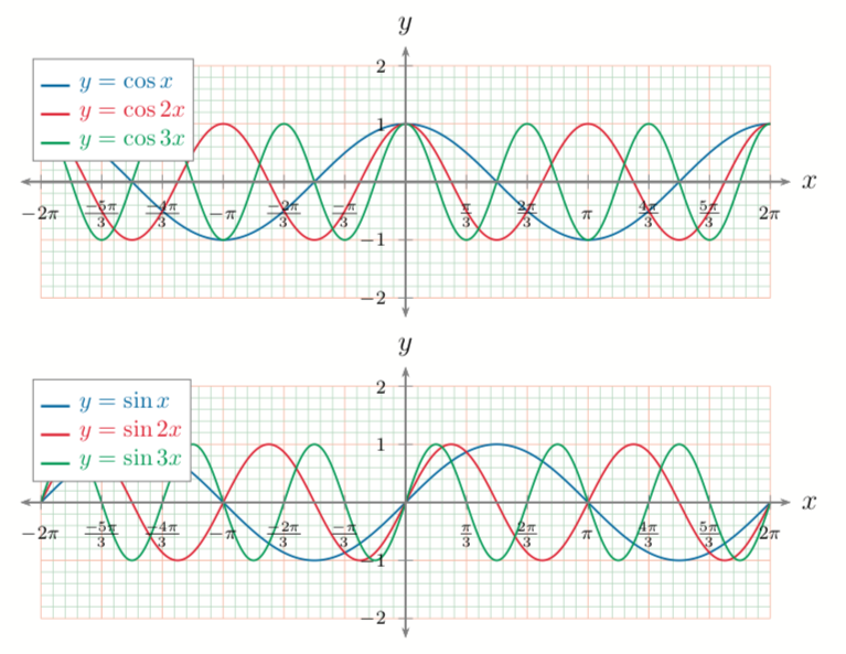
Integral of Orthogonal Functions

$\int_{-\pi}^{\pi} \cos (nt) \cos (mt) dt=\frac{1}{2}\int_{-\pi}^{\pi} \cos(n+m)t dt +\frac{1}{2}\int_{-\pi}^{\pi} \cos(n-m)t dt \ \ \ \ \ (2)$

This means that for ${n \neq m}$ :

$\int_{-\pi}^{\pi} \cos (nt) \cos (mt) dt= 0 \ \ \ \ \ (3)$

for ${n=m}$ :

$\int_{-\pi}^{\pi} \cos (nt) \cos (mt) dt= \pi \ \ \ \ \ (4)$

$\displaystyle \int_{-\pi}^{\pi} \sin (nt) \cos (mt) dt=\frac{1}{2}\int_{-\pi}^{\pi} \sin((n+m)t) dt +\frac{1}{2}\int_{-\pi}^{\pi} \sin((n-m)t) dt \ \ \ \ \ (5)$

This means for all value of ${m}$ that $\int_{-\pi}^{\pi} \cos (nt) \cos (mt) dt= 0 \ \ \ \ \ (6)$

$\displaystyle \int_{-\pi}^{\pi} \sin (nt)\sin (mt) dt=\frac{1}{2}\int_{-\pi}^{\pi} \cos((n-m)t) dt +\frac{1}{2}\int_{-\pi}^{\pi} \cos((n+m)t) dt \ \ \ \ \ (7)$

This means that for ${n \neq m}$ :

$\int_{-\pi}^{\pi} \sin (nt) \sin (mt) dt= 0 \ \ \ \ \ (8)$

for ${n=m}$ :

$\int_{-\pi}^{\pi} \sin (nt) \sin (mt) dt= \pi \ \ \ \ \ (9)$

Determination of ${a_0}$

We start to integrate both the members of the Fourier series from ${-\pi}$ to ${\pi}$

$\int_{-\pi}^{\pi} f(t)dt=\int_{-\pi}^{\pi}\left[\frac{a_0}{2}+\sum_{n=1}^{\infty}a_n \cos (nt)+\sum_{n=1}^{\infty}b_n\sin (nt) \right] dt$

$\int_{-\pi}^{\pi}f(t)dt=\frac{a_0}{2}\int_{-\pi}^{\pi}dt +\int_{-\pi}^{\pi} \left(\sum_{n=1}^{\infty}a_n\cos (nt)\right)dt+\int_{-\pi}^{\pi} \left(\sum_{n=1}^{\infty}b_n\sin (nt)\right)dt$

For the integrals formulas that we have derived before, we obtain

$\int_{-\pi}^{\pi}f(t)dt=\frac{a_0}{2}\int_{-\pi}^{\pi}dt +0 + 0=\pi a_0$

namely, $a_0=\frac{1}{\pi}\int_{-\pi}^{\pi} f(t)dt$

${A_0=a_0/2}$ is equal to the average value of the function ${f(t).}$

Determination of ${a_n}$

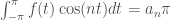
We start by multiplying both the members of the Fourier series by ${\cos (mt)}$ and then integrate from ${-\pi}$ to ${\pi}$

$\int_{-\pi}^{\pi} f(t)\cos (mt) dt=\int_{-\pi}^{\pi}\left[a_0+\sum_{n=1}^{\infty}a_n\cos(nt)+\sum_{n=1}^{\infty}b_n\sin (nt)\right]\cos (mt) dt$

Shall we consider the integrals that we get on the right-hand-side:

First term: $\int_{-\pi}^{\pi}a_0\cos (mt) dt =0$

The second integral for ${m=n}$ is equal to:

$\int_{-\pi}^{\pi} \sum_{n=1}^{\infty}a_n\cos (nt)\cos (mt) dt = a_n\pi$

The third integral for the orthonormality of the function is always equal to:

$\int_{-\pi}^{\pi} \sum_{n=1}^{\infty}b_n\sin (nt)\cos (mt) dt = 0$

Therefore:

$\int_{-\pi}^{\pi}f(t)\cos (nt) dt=a_n\pi$

namely, for ${m= 1, 2, 3, ...}$ :

$a_n=\frac{1}{\pi}\int_{-\pi}^{\pi}f(t)\cos (nt) dt$

Determination of ${b_n}$

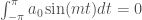
We start by multiplying both the members of the Fourier series by ${\sin(mt)}$ and then integrate from ${-\pi}$ to ${\pi}$

$\int_{-\pi}^{\pi}f(t)\sin(mt) dt=\int_{-\pi}^{\pi}\left[a_0+\sum_{n=1}^{\infty}a_n\cos(nt)+\sum_{n=1}^{\infty}b_n\sin (nt)\right]\sin(mt) dt$

Shall we consider the integrals that we get on the right-hand-side:

First term:

$\int_{-\pi}^{\pi}a_0\sin(mt) dt =0$

Second term:

$\int_{-\pi}^{\pi} \sum_{n=1}^{\infty}a_n\cos (nt)\sin(mt) dt = 0$

Third term:

$\int_{-\pi}^{\pi} \sum_{n=1}^{\infty}b_n\sin (nt)\sin(mt) dt = b_n\pi$

Therefore:

$\int_{-\pi}^{\pi}f(t)\sin(nt) dt=b_n\pi$

namely, for ${m= 1, 2, 3, ...}$ :

$b_n=\frac{1}{\pi}\int_{-\pi}^{\pi}f(t)\sin(nt) dt$

Summary

The coefficients of the Fourier series

By replacing m with n we can finally express the coefficient of the series in the final form.

$a_0=\frac{1}{\pi}\int_{-\pi}^{\pi}f(t)dt$

$a_n=\frac{1}{\pi}\int_{-\pi}^{\pi}f(t)\cos (nt) dt$

$b_n=\frac{1}{\pi}\int_{-\pi}^{\pi}f(t)\sin(nt) dt$ with ${n=1,2,3,...}$

or in the same way we can integrate in the interval ${0-2\pi}$ with the same result:

$a_0=\frac{1}{\pi}\int_{0}^{2\pi}f(t)dt$

$a_n=\frac{1}{\pi}\int_{0}^{2\pi}f(t)\cos (nt) dt$

$b_n=\frac{1}{\pi}\int_{0}^{2\pi}f(t)\sin(nt) dt$

For a given generic interval ${[-p,p]}$

$a_0=\frac{1}{p}\int_{-p}^{p}f(t)dt$

$a_n=\frac{1}{p}\int_{-p}^{p}f(t)\cos (\frac{n\pi t}{p}) dt$

$b_n=\frac{1}{p}\int_{-p}^{p}f(t)\sin(\frac{n\pi t}{p}) dt$ with ${n=1,2,3,...}$

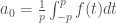
and the Fourier series is give by

$f(t)=\frac{a_0}{2}+\sum_{n=1}^{\infty}a_n\cos (\frac{n\pi t}{p})+\sum_{n=1}^{\infty}b_n\sin (\frac{n \pi t}{p})$

Example 1

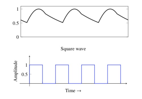
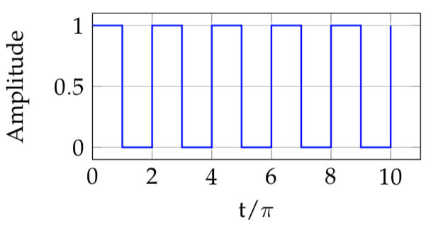
In this example, we will calculate the Fourier coefficient of a the square wave function. This function is of paramount importance in digital electronics since it used in the electronic signal to represent unit of information (bit) as on/off state.

Mathematically, the square wave is represented by functions as

$f(x)=\begin{cases} 1 & {0 < x <= \pi}, \\ 0 & \pi<x <= 2 \pi \end{cases}$

The plot of the extended periodic function is given in the following figure.

Figure 2: The function of the Exercise 1.

We now calculate the Fourier coefficients starting from the term $a_0$

$a_0 = \frac{1}{\pi} \int_{0}^{2\pi} f(t) ~dt$

$a_0 = \frac{1}{\pi} \left[\int_{0}^\pi f(t) ~dt +\int_{\pi}^{2\pi} f(t) ~dt \right]= 1.$

The coefficients $a_n$ are given by

$a_n= \frac{1}{\pi} \int_{-\pi}^{\pi} f(t) \cos(nt) dt =\frac{1}{\pi}\int_{0}^{\pi} {\pi} \cos(n)dt =0$ .

And finally

$\begin{aligned} b_n & = \frac{1}{\pi} \int_{-\pi}^\pi f(t) \sin (nt) ~dt \\ &= \frac{1}{\pi} \int_{0}^\pi \pi \sin (nt) ~dt \\ &= \left[ \frac{- \cos (nt)}{n} \right]_{t=0}^\pi \\ &= \frac{1 - \cos (\pi n)}{n} \\ &= \frac{1 - {(-1)}^n}{n}\end{aligned}$

$b_n=\begin{cases} \frac{2}{n} & \text{if } n \text{ is odd} , \\0 & \text{if } n \text{ is even} \end{cases}$

The Fourier series is

$f(t)=\frac{\pi}{2} + \sum_{\substack{n=1\\n \text{ odd}}}^{\infty} \frac{2}{n} \, \sin (n t)= \frac{\pi}{2} + \sum_{k=1}^{\infty} \frac{2}{2k-1} \, \sin \bigl( (2k-1)\, t \bigr)$ .

In this way, for example, the first 3 harmonics of the series are

$f(t)= \frac{\pi}{2} +2 \, \sin (t)+\frac{2}{3} \, \sin (3t)+ \cdots$

Example 2

In this second example the square wave signal is defined as a odd function such that $f(x)=-f(-x)$ and mathematically, the square wave is represented by functions as

$f(x)=\begin{cases} -1 & {-\pi < x <= 0}, \\ 1 & 0<x <= \pi \end{cases}$

The plot of the extended periodic function is given in the following figure.

Figure 3: The function of the Exercise 2.

We now calculate the Fourier coefficients starting from the term $a_0$

$a_0 = \frac{1}{\pi} \int_{-\pi}^\pi f(t) ~dt = \frac{1}{\pi} \int_{0}^\pi \pi ~dt = \pi .$

The coefficients $a_n$ are given by

$a_n= \frac{1}{\pi} \int_{-\pi}^{\pi} f(t) \cos(nt) dt =\frac{1}{\pi}\int_{0}^{\pi} {\pi} \cos(n)dt =0$ .

And finally

$b_n=\begin{cases} \frac{2}{n} & \text{if } n \text{ is odd} , \\0 & \text{if } n \text{ is even} \end{cases}$

The Fourier series is

$f(t)=\frac{\pi}{2} + \sum_{\substack{n=1\\n \text{ odd}}}^{\infty} \frac{2}{n} \, \sin (n t)= \frac{\pi}{2} + \sum_{k=1}^{\infty} \frac{2}{2k-1} \, \sin \bigl( (2k-1)\, t \bigr)$ .

The plot of the first 100 terms of the series is given in the following animation.

Figure 4: Animation showing the first 100 terms of the Fourier series for the square wave curve of Example 2. The animation was generated using a Gnuplot script available to this interesting website.

The overshoting oscillations in correspondence of the discontinuity of the square wave is called Gibbs phenomenon by W. Gibbs that pointed it out in a letter to Nature in 1899. The oscillation overshoot the function of a fixed amount that can be calculated. In addition, the function oscillate with an amplitude that is decreating going far from the discontinuity point.

Fourier Series using Complex Notation

Let ${f(x)}$ be a piecewise linear function on ${[-L,L]}$ (This means that ${f(x)}$ may possess a finite number of finite discontinuities on the interval). Then ${f(x)}$ can be expanded in a

$f(x)=\frac{a_0}{2}+\sum_{n=1}^{\infty} \left[ a_n\cos \frac{n\pi x}{L}+b_n\sin\frac{n\pi x}{L} \right] \ \ \ \ \ (10)$

Using Euler’s identities:

$\begin{aligned} \cos \theta &=& \frac{e^{i\theta}+e^{-i\theta}}{2}\\ \sin \theta &=& \frac{e^{i\theta}-e^{-i\theta}}{2i} \end{aligned}$

where ${i=\sqrt{-1}}$ ,

the Fourier series of ${f(x)}$ can be written in a more compact from as

$\displaystyle f(x) = \sum_{n=-\infty}^{\infty} c_n e^{i n\pi x/L} \ \ \ \ \ (11)$

where

$c_n = \frac{1}{2L} \int_{-L}^{L} f(x)e^{-in\pi x/L}dx \ \ \ \ \ (12)$

$\displaystyle c_n=\begin{cases} (a_n-b_n)/2 & n<0 \\ (a_n+b_n)/2 & n>0 \\ a_0/2 & n=0 \end{cases}$

The Discrete Fourier Transform (DFT)

IN CONSTRUCTION

Appendix I

A program in Awk language to calculate the DFT.

This program read a file containing a list of values representing a function or a signal or a generic set of data to analyze using the harmonical analysis. Then it calculates the Fourier coefficients and finally reconstructs the Fourier series using a given number of terms (n).

[code language="cpp"]
#==========================================================
#
# NAME: dft.awk
#
#==========================================================
# DESCRIPTION: Calculate the fourier series of a signal
# INPUT: The program read a two column file containing the
#        signal to elaborate
# OUTPUT: The output contain the reconstructed signal 
#         using the first n Fourier components.
#==========================================================
# DEVELOPED USING: gawk
# FUNCTIONS:
# ReadData()    : read a two column data file from stdin
# CalculateDFT(): Calculate the DFT.
# Reconstruct() : Reconstruct/filter the signal using the 
#       first n components of the DFT, and print on the 
#       stdout thereconstructed signal.
#==========================================================
# Author: Danilo Roccatano
# Version: 1.0
# Copyright (C): 2016 Danilo Roccatano
#==========================================================
#
#

function ReadData() {
#
# Read data from standard input
#
    np=0
    while (getline > 0 ) {
        if (NF >0) {
            P[np]=$2
            np++
        }
    }
    np--
}

function CalculateDFT() {
#
# Perfrom the discrete fourier transform of the data
#
    PI=4*atan2(1,1)
    for (j=1;j<=n;j++) {
        A[j]=0
        B[j]=0
        for (i=0;i<=np-1;i++) {
            x=2*PI*i*j/np
            A[j]+=P[i]*cos(x)
            B[j]+=P[i]*sin(x)
        }
        A[j]/=(np/2)
        B[j]/=(np/2)
    }
}
function CalcA0(){
#
# Calculate the average value of A0
#
    A0=0
    for (i=0;i<=np;i++) {
        A0+=P[i]
    }
    A0=A0/np
}
function Reconstruct() {
    for (i=0;i<=np;i++){
        M[i]=0
        for (j=1;j<=np;j++) {
            F=2*PI*j*i/np
            M[i]=M[i]+A[j]*cos(F)+B[j]*sin(F)
        }
        print i,M[i]+A0
    }
}
BEGIN {

#
# n:= number of armonics to consider
#
n=30
    ReadData()
    CalcA0()

    CalculateDFT()
#
# Reconstruct the signal using n harmonics
#
    Reconstruct()

}
[/code]

Appendix II

A program in tcl/tk language for the harmonic analysis of a drawn signal

This program was inspired to a similar program in BASIC language in a book that I read many years ago [1]. Using the mouse, you can draw a function in the upper canvas, calculate numerically the Fourier coefficients and plot a number of terms to your choice of the discrete Fourier series.

[code language="bash"]
#! /bin/sh
# the next line restarts using wish \
exec wish "$0" "$@"
#==========================================================
# NAME: FourierV3.0.tcl
#==========================================================
# DESCRIPTION: Perfrom the harmonic analysis of a drawn  
# signal. 
#==========================================================
# DEVELOPED USING: tcl/tk
#==========================================================
# Author: Danilo Roccatano (c) 2018
# Version: 3.0
#==========================================================
#
#

package require Tk
package require xyplot
package require Plotchart

wm title . ""

array set Yv {}
array set Yvt {}
array set A {}
array set B {}
array set P {}

set width 1000
set height 200
set midX  [expr { $width/2 }]
set midY  [expr { $height/ 2 }]
set imidY [expr { 1.0/ $midY }]
set xsta 0
set xend 0
set x0 0
set y0 0
set np $width
set np1 [expr $np-1]
set np2 [expr $np/2]
set inp2 [expr 1.0/$np2 ]
set n  10
set A0  0

set pi 3.1415926535897931
set K 2*$pi/$np
set COLORS {
    navy 
    cyan 
    green chartreuse 
    gold 
    chocolate 
    red 
    magenta 
    purple 
    blue 
    turquoise
    aquamarine
    yellow
    sienna 
    peru 
    burlywood 
    wheat
    tan 
    firebrick 
    brown 
    salmon
    orange 
    coral 
    tomato
    pink 
    maroon 
    violet 
    orchid 
    lavender 
    }
set nCOLORS [llength $COLORS]
set icol 0
puts "$nCOLORS" 

global xsta xend  width  height midY K inp2 imidY A0 COLORS icol

for { set i 1 } { $i <= $width+10 } { incr i 1 } {
    set Yv($i) [expr {  $midY } ]
    set P($i) 0 
    set Yvt($i)  0 
    set A($i)  0 
    set B($i)  0 
   }

proc DrawAxis {w} {
       global width height midY

       $w create line 0 $midY  $width   $midY  -tags "Xaxis"  -fill black -width 1
}

proc redraw {w ar1 ar2 ar3 x y} {
    upvar $ar1 Yv
    upvar $ar2 Yvt
    upvar $ar3 P
    global  xsta xend  width K midY imidY A0 np
    set x0 0
    set y0 0
    set icol 0
    $w delete "all"
    DrawAxis .c

    set A0  0
    for { set x $xsta } { $x <= $xend   } { incr x 1 } {
        set ix [expr int($x)]
        set Yv($ix) 0 
        set Yv($ix) $Yvt($x) 
        set Yvt($ix) 0 
   }

   set A0 [expr $A0/$np]
   set y0 0
   for { set x 1 } { $x <= $width } { incr x 1 } {
       set ix [expr int($x)]
       if {$Yv($ix) != 0 } { 
           $w create line $x0 $y0  $x  $Yv($ix)  -fill red -width 1
           set x0 $x
           set y0 $Yv($ix)
      } 
      if {$Yv($ix) == 0 } {
        set Yv($ix) $y0
      }
        set P($ix) [expr -($Yv($ix)-$midY)*$imidY]
   }
}

proc down {w Yv Yvt x y} {
    global xsta x0 y0
    set ::ID  [$w create line $x $y $x $y -fill black]
    set xsta $x
    set x0 $x
    set y0 $y
}

proc move {w ar  x y} {
     upvar $ar Yvt
     global  xend xsta x0 y0
     set x [$w canvasx $x]
     set y [$w canvasx $y]
     $w create line $x0 $y0 $x $y -fill black 
     set xend $x
     set ix [expr int($x)]
     set Yvt($ix) $y
     set x0 $x
     set y0 $y
 }

proc DFT {w w1 w2 n ar1 ar2 ar3 ar4} {
     #
     # Perfrom the discrete fourier transform of the data
     #
     upvar $ar1 A 
     upvar $ar2 B 
     upvar $ar3 Yv
     upvar $ar4 P
     global pi np np1  np2 inp2 K midY A0 icol
     puts "Calculating the coefficients ...  "
    
     for { set j 1}  {$j <= $n} {incr j 1} {
         set A($j) 0
         set B($j) 0
         for { set i 1}  {$i <= $np} {incr i 1} {
             set x [expr $K*($i-1)*$j]
             set A($j) [expr $A($j)+$P($i)*cos($x)]
             set B($j) [expr $B($j)+$P($i)*sin($x)]
         }
         set A($j)  [expr $A($j)*$inp2]
         set B($j)  [expr $B($j)*$inp2]
    }
    PlotPSpect $w1 $w2 $n A B
    puts "Reconstructing the signal using $n harmonics"
    set icol [expr $icol +1]
    if {$icol > 29} {set icol 0}
    RecSignal $w $n A B 
}

proc RecSignal {w n ar1 ar2 } {
    upvar $ar1 A 
    upvar $ar2 B 
    set x0 0 
    set y0 0     
    global pi np midY K A0 COLORS icol
    for { set i 1}  {$i <= [expr $np+1]} {incr i 1} {
        set M($i) 0 
        for { set j 1}  {$j <= $n} {incr j 1} {
            set x [expr $K*($i-1)*$j]
            set M($i) [expr $M($i)+$A($j)*cos($x)+$B($j)*sin($x)]
        }
        set M($i) [expr $midY-$M($i)*$midY]
        $w create line $x0 $y0  $i  $M($i)  -fill [lindex $COLORS $icol] -width 1
        set x0 $i
        set y0 $M($i)
    }
}

proc ClrCanvas {w } {
    $w delete "all"
    set icol 0
    DrawAxis $w 
}

proc PlotPSpect {w1 w2 n ar1 ar2} {
    upvar $ar1 A 
    upvar $ar2 B 
    set xval {}
    global pi 
    $w1 delete all
    $w2 delete all
    set p  [::Plotchart::createHistogram $w1 {0 30 2} {0 1.0 0.1}]
    set p1 [::Plotchart::createXYPlot $w2 {0 30 2} {-180. 180 30 }]
    $p title "Power Spectrum" 
    $p xtext "# harmonics" 
    $p dataconfig data  -fillcolour cyan -width 2 -colour blue 
    $p1 dataconfig data  -fillcolour cyan -width 2 -colour red -type symbol 
    $p1 title "Phase angle" 
    $p1 xtext "# harmonics" 

    for { set i 1 } { $i <= $n } { incr i } {
      $p plot data $i [expr sqrt($A($i)*$A($i)+$B($i)*$B($i))]
      $p1 plot data $i [expr -atan2($B($i),$A($i))*180./$pi]
      puts "$i [expr -atan2($B($i),$A($i))]"
#     puts "$A($i)  $B($i)"
    }
}

#
#-- Building the UI
set colors { black red orange }
label .ltitle \
-background magenta -padx 64 -relief raised -text {Harmonic Analysis      (c) Danilo Roccatano 2002-2018}

set xyp [xyplot .xyp -xformat "%5.0f" -yformat "%5.4f" -title "Power Spectrum" -background gray90]
button  .b1    -text FOURIER      -command { DFT .c .c1 .c2 $n A B Yv P}
scale .scale -orient horizontal  -length 300 -from 1 -to 30 \
    -tickinterval 3 -variable n 
label .lscale -text "      Harmonics"   

label .descr -justify left -background pink -padx 32 -relief raised -wraplength 800 -text {Calculation of the discrete Fourier Harmonics of a generic curve drawn in the above canvas.  Use the mouse pointer to draw a curve. Everytime you click on the canvas the new curve will be merged with the existent one.  Once you you finish, select the number f harmonics to consider for the curve reconstruction (defauls 10) and then press FOURIER button. The program calculate also the power spectrum and the phase angle for each harmonic term of the series. HAVE FUN!}

button  .b2   -text "Clear All" -padx 20 -pady 20 -command { ClrCanvas  .c }

canvas .c -relief raised -borderwidth 1 -width 1000 -height 200 \
-background white -relief raised -border 2 

pack [canvas .c1 -width 400 -height 300 -bg white]
pack [canvas .c2 -width 400 -height 300 -bg white]

grid .ltitle -row 0 -columnspan 4 -sticky news
grid .descr    -row 1 -columnspan 4 -sticky news  
grid .c  -row 2  -columnspan 4 -sticky news 
grid .c1  -row 3  -columnspan 2 -columnspan 2 -sticky news
grid .c2  -row 3 -column 3  -columnspan 2 -sticky news
grid .b1  -row 4 -column 0   -sticky w
grid .b2  -row 4 -column 1   
grid .lscale -row 4 -column 3 -sticky e
grid .scale  -row 4 -column 3   -sticky nw

#-- The current mode is retrieved at runtime from the global ''Mode'' variable:
bind .c <1>         {down %W Yv Yvt %x %y}
bind .c <ButtonRelease-1>  {redraw %W Yv Yvt P %x %y }
bind .c <B1-Motion> {move %W Yvt %x %y}
bind .c <3>         {%W delete current}
 
DrawAxis .c

[/code]

"… I seem […] only like a boy playing on the sea-shore, and diverting myself in now and then finding a smoother pebble or a prettier shell than ordinary, whilst the great ocean of truth lay all undiscovered before me". – Isaac Newton.