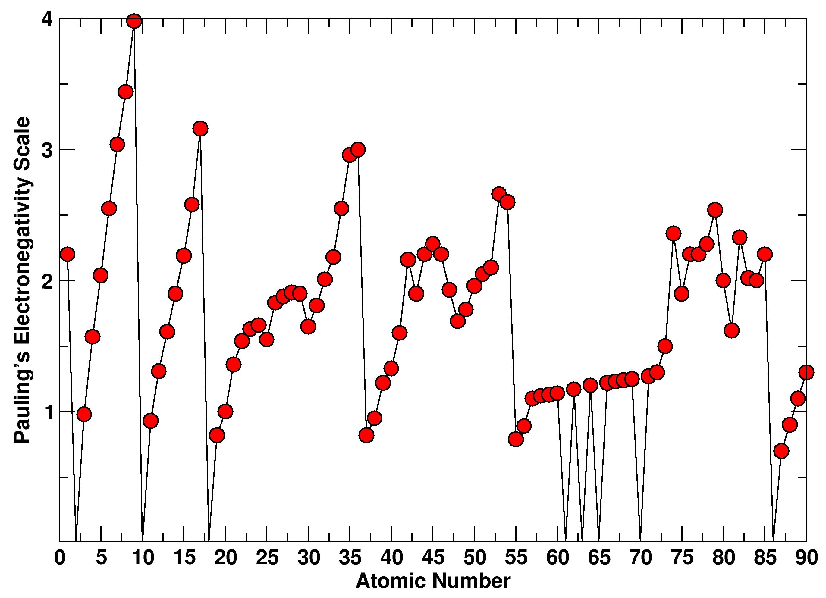
The electronegativity of a chemical element measures the tendency of an atom to attract electrons around it. This definition was formalized for the first time, in a semi-empirical form, by the chemist Linus Pauling in the early 1930s, but it had already been proposed in the late 1800s by the Swedish chemist Berzelius. In molecules, this tendency determines the molecular electronic distribution and therefore influences molecular properties such as the distribution of partial charges and chemical reactivity. Pauling provided an electronegativity scale by comparing bond dissociation energies of pairs of atoms (A, B) using the equation

With $E_{AB}$, $E_{AA}$, and $E_{BB}$ being the dissociation energies of the molecules AB, AA, and BB, respectively.

A few years later, in 1934, Mulliken proposed an expanded definition of electronegativity based on spectroscopically measurable atomic properties such as ionization potential (I) and electron affinity (E):

The ionization potential and electron affinity are defined as follow:

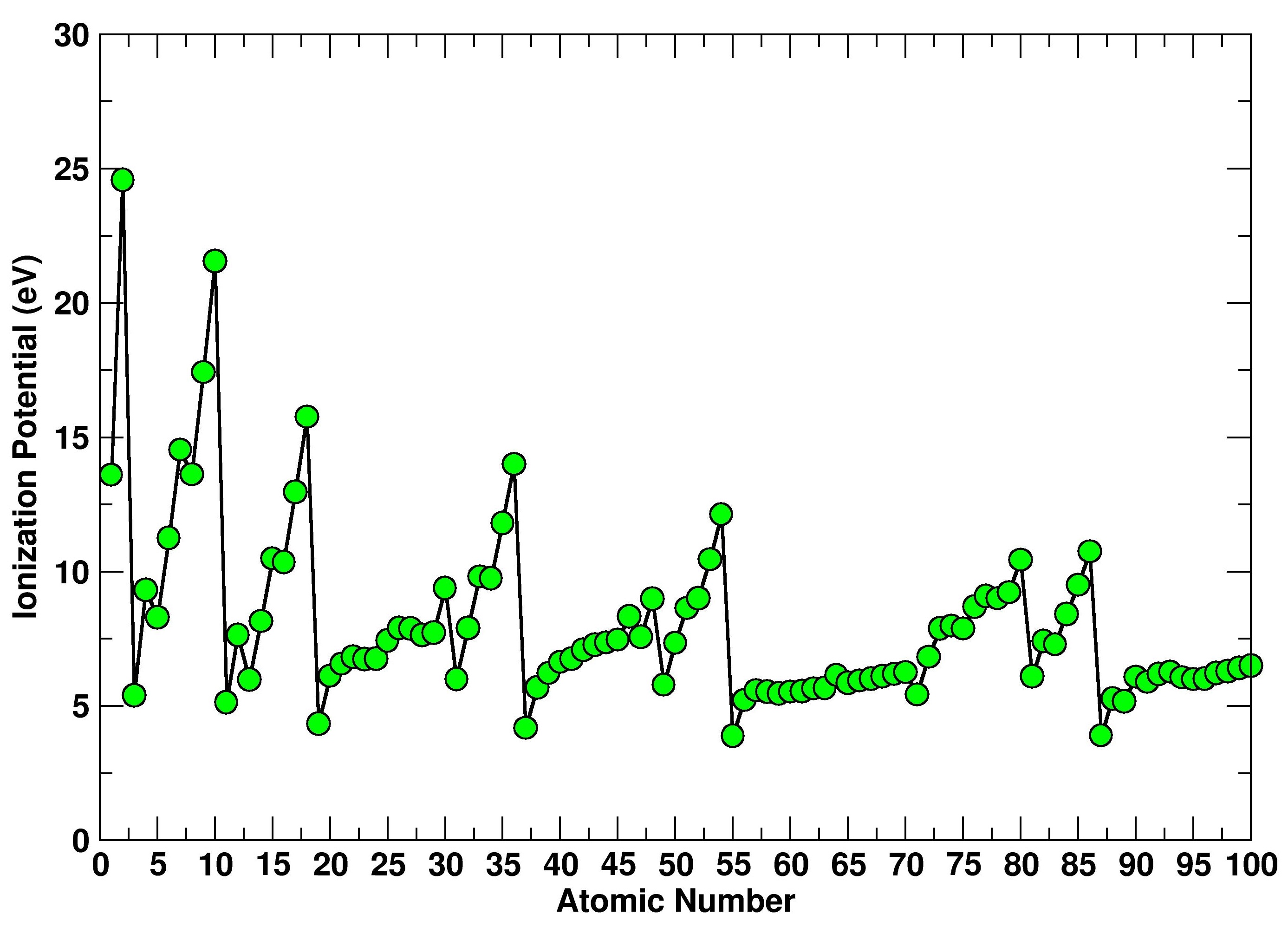
1. Ionization Energy: Ionization energy is the energy required to remove an electron from an atom or a positive ion. In other words, it represents the amount of energy needed to convert a neutral atom into a positive ion. Ionization energy is measured in electronvolts (eV) or joules per mole (J/mol). In the Figure below the ionization potentials of the first 100 elements of the periodic table are reported. For example, the ionization energy of hydrogen is about 13.6 eV, which means that at least 13.6 eV of energy must be supplied to remove an electron from a hydrogen atom and convert it into an H+ ion. Ionization Energy of Sodium (Na): Approximately 5.1 eV (or 495 kJ/mol). This value represents the energy required to remove an electron from a sodium atom to form an Na+ ion.
2. Electron Affinity: Electron affinity is the energy released when an atom or ion captures an electron to form a negative ion (anion). In other words, it represents the amount of energy released when an atom gains an additional electron. Electron affinity is also measured in electronvolts (eV) or joules per mole (J/mol). For example, the electron affinity of chlorine is about -349 kJ/mol, which means that chlorine releases energy when it captures an electron to become a Cl- ion. Electron Affinity of Oxygen (O): Approximately -141 kJ/mol. This value represents the energy released when an oxygen atom captures an electron to form an O2- ion.

In the table below, the electronegativities of hydrogen and atoms of the second period obtained from these two definitions are compared.

Atom
H	2.20	3.059
Li	0.91	1.282
Be	1.57	1.987
B	2.04	1.828
C	2.55	2.671
N	3.04	3.083
O	3.44	3.215
F	3.98	4.438

The use of electronegativity to calculate molecular properties, such as charge distribution, was first proposed by Robert Thomas Sanderson in 1951. The proposed method is based on the concept of electronegativity equalization in atoms within molecules. The basic idea is to assume that when two or more atoms with initially different electronegativities chemically combine, electrons redistribute until a constant average electronegativity value of the compound is reached. This molecular electronegativity is calculated as the geometric mean (the geometric mean of n numbers is obtained by multiplying all the numbers together and taking the n-th root of the product) of the electronegativity values of the atoms composing the compound. In other words, electron density redistributes from the most electronegative atom to the most electropositive atom, creating a partial positive charge on the former and a partial negative charge on the latter. As the positive charge on the electropositive atom increases, its effective nuclear charge increases, thus increasing its electronegativity. The same trend occurs in the opposite direction for the most electronegative atom, until both atoms have the same electronegativity.

The concept of electronegativity balancing is rooted in the definition of Electron Chemical Potential proposed by Parr. Parr’s Electron Chemical Potential (μ) is a scalar quantity associated with the electron density of a chemical system and represents the Helmholtz free energy to add or remove an electron particle from a specific region of the system while keeping the total electron density constant. In simpler terms, Parr’s Electron Chemical Potential measures the energy required to change the electron density in a specific region of a chemical system. This concept is useful for understanding how variations in electron density influence chemical reactions and the properties of molecular systems. The general formula for Parr’s Electron Chemical Potential (μ) can be expressed as:

​

Where:

• is the electronic chemical potential of Parr.
• E is the total energy of the system.
• N is the total number of electrons.

This way electronegativity is identified with a thermodynamic potential. Atomic electronegativity is considered as the gradient of thermodynamic activity of electrons. Electrons moving along this gradient change the value of the total electronegativity of the molecule to an intermediate value between those of the isolated atoms. This definition was then extended in 1962 by Hinze and Jaffe to electrons in molecules, with the introduction of orbital electronegativity. This definition takes into account the state of electrons in molecular orbitals, which depends on the hybridization and the occupancy state of these orbitals. The difference in charge density of an atom A in its isolated state and that inside the molecule is interpreted in terms of the partial charge present in the orbital of atom A. Therefore, it is possible to have a relationship between the value of the partial charge of each atom and its electronegativity value.

The Sanderson Method

Let’s delve into what the Sanderson method entails. The concept of electronegativity equalization assumes that the differences in electronegativity between atoms in a molecule should be minimized. This approach provides a simple and intuitive way to estimate partial charges without the need for complex calculations. Sanderson proposed an electronegativity scale (S) based on Mulliken’s, taking into account the compactness of the atom. He also calculates the change in electronegativity per unit charge for each atomic species as:

The method assigns partial charges to atoms based on their electronegativity values and the geometric mean electronegativity of their bonded neighbors.

For example, the electronegativity of phosphorus oxyfluoride (POF3) is the fifth root of the product (Sanderson electronegativity scale).

To calculate the charges on each atom of the compound, we need to consider the electronegativities of the atoms composing the molecule.

Atom	S
P	2.515	2.490
O	3.654	3.ooo
F	4.00	3.140

The partial charges are then calculated as follows:

We can now verify the correctness of the calculation by evaluating the total charge of the molecule:

The Sanderson method provides a quick and simple approach to estimate partial charges based on electronegativity equality. However, using the Sanderson total equilibration method to obtain orbital electronegativity values in a molecule leads to unrealistic results, as the method does not consider the molecular structure, but only connectivity. A classic example is that of conformational isomers, molecules with the same number of atoms and bonds but arranged in different structures. To overcome these issues, other methods have been proposed that take into account the type of chemical bonding of each atom in the molecule. We will see how these methods work in the next article of this series.

References

1. D. Bergman and J. Hinze. Electronegativity and Molecular Properties. Angew. Chem. Int. Ed. Engl. 1996, 35, 150-163.
2. R.T. Sanderson. Science. 1951,114, 670-672.
3. R. T. Sanderson. Principles of Electronegativity. Part I. J. Chem Edu., 1988, Vol: 65 (2), pp 112.
4. R. T. Sanderson. Principles of Electronegativity. Part II. J. Chem Edu., 1988, Vol: 65 (3), pp 227.