Boundary value problems (BVPs) for ordinary differential equations arise naturally in many areas of physics, engineering, and applied mathematics. Classical examples include the vibration of strings, heat conduction in solids, and quantum mechanical bound states. Unlike initial value problems (IVPs), where all conditions are specified at a single point, BVPs impose constraints at different points of the domain, making them significantly more challenging to solve both analytically and numerically.
The shooting method is one of the most intuitive and historically rooted techniques for tackling such problems. Its central idea is simple: transform a boundary value problem into an initial value problem by guessing the missing initial conditions, then iteratively refine this guess until the solution satisfies the boundary conditions at the other end. The method is often illustrated through a ballistic analogy—one “shoots” from the initial point and adjusts the trajectory until the target is hit. Although the shooting method was formalized only in the 20th century, its conceptual foundations can be traced back much earlier. The study of differential equations in the 18th and 19th centuries by mathematicians such as Leonhard Eulerand Joseph-Louis Lagrange already revealed the difficulty of boundary value problems in mechanics and astronomy. At that time, analytical solutions were often unavailable, and practitioners relied on approximation strategies that implicitly resembled “trial-and-error” approaches. A decisive step toward the modern shooting method came with the development of reliable numerical solvers for initial value problems around 1900, notably through the work of Carl Runge and Martin Kutta. Their methods provided the computational backbone needed to integrate differential equations accurately from a given starting point. This made it feasible to implement the idea of repeatedly “shooting” with different initial guesses. The method gained wider recognition and systematic treatment in the mid-20th century, alongside the emergence of numerical analysis as a distinct discipline. Influential mathematicians such as Richard Courant contributed to the theoretical understanding of boundary value problems, while the increasing availability of digital computers transformed the shooting method into a practical and widely used computational tool.
Today, the shooting method remains a cornerstone in the teaching of numerical methods due to its conceptual clarity and direct connection to physical intuition. While more robust techniques—such as finite difference and finite element methods—are often preferred for complex or stiff problems, the shooting method continues to play an important role in applications ranging from classical mechanics to quantum physics, where it is frequently used to determine eigenvalues and admissible solutions.
In this blog, I will give an example of the application of the method to the solution of the Thomas-Fermi and Thomas-Fermi-Dirac equations.
The Shooting Method
The Shooting Method is commonly used to solve ODEs of the form:

These ODEs often arise in physics, engineering, and other fields to model various physical phenomena.
To uniquely determine a solution, you need to specify boundary conditions at two different points within the domain, typically at 


These conditions define the values of the dependent variable (y) at the boundary points. The Shooting Method approaches the BVP by transforming it into an initial value problem (IVP). It starts with an initial guess for the derivative (

solve_ivp function in Python. The IVP solution provides the values of (y) and (
You evaluate this solution at (

The Iterative Process:
- If the solution at (
- You continue this iterative process until the solution at (
- The iteration can be guided by a numerical root-finding method (e.g., bisection or Newton’s method) to refine the guess for (
The method converges when the IVP solution at (
The Shooting Method is versatile and can be applied to various ODEs with boundary conditions. It’s especially useful when other methods like finite difference methods or spectral methods are not suitable. It can require multiple iterations to find the correct initial condition, and the convergence may not be guaranteed for all problems. The choice of initial condition and the convergence behavior can depend on the specific problem being solved.
EXAMPLE: THE THOMAS-FERMI-DIRAC EQUATION
The Thomas–Fermi–Dirac (TFD) approach belongs to a class of models in which the behavior of many-electron systems is described in terms of continuous densities rather than individual wavefunctions. Historically, it represents one of the earliest attempts to move from a fully quantum-mechanical description to a more tractable, statistical one. At its core, the method assumes that electrons in an atom or solid can be treated as a degenerate Fermi gas locally in equilibrium, so that their properties depend only on the local value of the potential. This leads to nonlinear differential equations for an effective potential or density.
It is important to note, however, that the equation written above,

is structurally a Schrödinger-type equation, rather than the genuine Thomas–Fermi–Dirac equation. In this context, it can be interpreted as an effective one-particle equation used in a shooting method framework, where the term E_f plays the role of a reference (Fermi) energy. The actual Thomas–Fermi–Dirac equation is nonlinear and typically written in terms of a dimensionless potential \phi(x), with a characteristic structure of the form:

where the first term arises from the kinetic energy of the electron gas, and the second term represents the Dirac exchange correction. This nonlinearity is what gives rise to the rich behavior we observed numerically, including the appearance of a local maximum (“bump”) in the solution.
Before the inclusion of exchange effects, the simpler Thomas–Fermi (TF) model already provided a remarkable description of electron distributions using only the local electron density. In that case, the equation retains only the kinetic contribution and leads to a monotonically decaying solution, reflecting a purely repulsive “pressure-like” behavior of the electron gas.
The addition of the Dirac term in TFD introduces an effective attractive correction, fundamentally altering the structure of the solution. This difference will be explored in more detail—both analytically and numerically—in a separate post dedicated specifically to the Thomas–Fermi model and its physical implications.
From a modern point of view, the Thomas–Fermi and Thomas–Fermi–Dirac models can be seen as early precursors of density-based approaches, where the complexity of many-body quantum mechanics is reduced to equations for continuous fields. Despite their simplicity, these models already capture essential physical mechanisms such as screening, collective behavior, and the balance between kinetic and interaction effects.
To solve this equation numerically, we can use the finite difference method, which replaces derivatives with discrete approximations on a grid.
The general steps are as follows:
The first step is to define the domain of interest and discretize it into N points:

Then, you choose boundary conditions for $latexf(x).$ For example, in bound-state problems one typically imposes:

Hence, you define the potential energy function 


You also need to define the step size 

You are now ready to apply the finite difference approximation to the second derivative: 

The process is then iterated over the grid to compute f(x), starting from the initial values 

The solution is then normalized, typically imposing: 
DESCRIPTION OF THE PROGRAM
The main purpose of this code is to numerically solve the Thomas–Fermi–Dirac equation, which describes the spatial distribution of fermions (such as electrons) in a given potential. The shooting method is used to determine the solution that satisfies the boundary conditions, allowing one to obtain a physically meaningful density profile. The resulting solution is then plotted to visualize how the particles are distributed in the system.
The program also includes the classical Thomas–Fermi (TF) model, enabling a direct comparison between the two approaches. While the TF model accounts only for the kinetic contribution of the electron gas, the Thomas–Fermi–Dirac (TFD) model incorporates an additional exchange term, which leads to qualitative differences in the solution.
The numerical integration is performed using the function solve_ivp from SciPy, which provides an efficient solver for systems of ordinary differential equations. The second-order equation is rewritten as a system of first-order equations and integrated over a discretized spatial domain.
A central role is played by the implementation of the shooting method. Starting from one boundary, the differential equation is integrated forward using an initial guess for the slope. This guess is then iteratively refined until the solution satisfies the required boundary condition at the opposite end of the domain. In this way, the boundary value problem is reduced to a sequence of initial value problems.
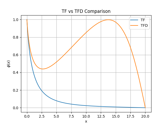
By solving the equation for both the TF and TFD models, the program highlights the impact of the exchange interaction. In particular, while the Thomas–Fermi solution exhibits a smooth monotonic decay, the inclusion of the Dirac term in the TFD model can lead to a non-monotonic behavior, with the appearance of a characteristic maximum (see Figure above).
APPENDIX
The Python code
"""
===========================================================
Thomas–Fermi vs Thomas–Fermi–Dirac Equation Solver
===========================================================

Description:
    This program numerically solves the Thomas–Fermi (TF) and
    Thomas–Fermi–Dirac (TFD) equations using a simple shooting method.

    The Thomas–Fermi model provides a statistical description of the
    electron density in atoms based on kinetic effects only. The
    Thomas–Fermi–Dirac extension includes the Dirac exchange term,
    introducing an additional interaction that modifies the solution.

Method:
    - The nonlinear second-order differential equation is rewritten
      as a system of first-order equations.
    - A shooting method with bisection is used to determine the
      correct initial slope.
    - The ODE is integrated using scipy.integrate.solve_ivp.

Features:
    - Direct comparison between TF and TFD solutions
    - Minimal and readable implementation
    - Suitable for educational and illustrative purposes

Output:
    A plot comparing the TF and TFD solutions, highlighting the
    qualitative effect of the exchange term (e.g., non-monotonic behavior).

Notes:
    - The equation is singular at x = 0; integration starts from a
      small value eps.
    - This is a simplified implementation intended for demonstration.

===========================================================
#  Author: D. Roccatano
#  This code was developed with the assistance of OpenAI ChatGPT
#  (version GPT-5.3, 2026) for code generation and explanations.
#
#  Date: 2025
#  License: MIT
================================================================

"""

import numpy as np
import matplotlib.pyplot as plt
from scipy.integrate import solve_ivp

# -----------------------------
# SETTINGS
# -----------------------------
model = "TFD"   # "TF" or "TFD"
lam = 0.3       # used only for TFD

x_max = 20.0
N = 2000
eps = 1e-6

x_grid = np.linspace(eps, x_max, N)

# -----------------------------
# ODE definition
# -----------------------------
def tf_ode(x, y):
    phi, dphi = y

    if phi < 0:
        phi = 0

    # Base Thomas-Fermi term
    d2phi = phi**1.5 / np.sqrt(x)

    # Add Dirac correction if selected
    if model == "TFD":
        d2phi -= lam * phi

    return [dphi, d2phi]

# -----------------------------
# Shooting function
# -----------------------------
def shoot(slope):
    y0 = [1.0 + slope*eps, slope]

    sol = solve_ivp(
        tf_ode,
        [eps, x_max],
        y0,
        t_eval=x_grid,
        method='RK45'
    )

    phi_end = sol.y[0][-1]
    return phi_end, sol

# -----------------------------
# Bisection shooting
# -----------------------------
def find_solution():
    s1, s2 = -10.0, -0.01

    f1, _ = shoot(s1)
    f2, _ = shoot(s2)

    if f1 * f2 > 0:
        raise RuntimeError("Bad initial slope guesses.")

    for _ in range(60):
        sm = 0.5*(s1 + s2)
        fm, sol = shoot(sm)

        if abs(fm) < 1e-6:
            break

        if f1 * fm < 0:
            s2, f2 = sm, fm
        else:
            s1, f1 = sm, fm

    return sol

# -----------------------------
# Solve
# -----------------------------
solution = find_solution()
phi = solution.y[0]

# -----------------------------
# Plot
# -----------------------------

results = {}

for model_name in ["TF", "TFD"]:
    model = model_name
    solution = find_solution()
    results[model_name] = solution.y[0]

# Plot comparison
for key, phi in results.items():
    plt.plot(x_grid, phi, label=key)

plt.xlabel("x")
plt.ylabel(r"$\phi(x)$")
plt.title("TF vs TFD Comparison")
plt.legend()
plt.grid()
plt.show()


Pingback: Ettore Majorana e L’Equazione di Fermi-Thomas |