The Smoluchowski Diffusion Equation |

The Smoluchowski diffusion equation describes the time evolution of the probability density function (PDF) of a particle undergoing overdamped Brownian motion in a potential energy landscape. It is a central equation in statistical mechanics, soft matter physics, and chemical physics.

Its origins trace back to the early 20th century, in the context of the theoretical understanding of Brownian motion. Following the seminal work of Albert Einstein in 1905, who provided a statistical description of diffusion and established a quantitative link between microscopic fluctuations and macroscopic transport, further developments aimed to incorporate external forces and interactions. In 1916, Marian Smoluchowski extended Einstein’s framework by considering particles subjected to systematic forces arising from a potential field. His formulation led to what is now known as the Smoluchowski equation, effectively describing diffusion in the overdamped (high-friction) limit where inertial effects can be neglected. This marked a crucial step toward connecting stochastic motion with deterministic drift. A complementary perspective emerged through the work of Paul Langevin (1908), who introduced a stochastic differential equation for particle motion, explicitly incorporating random forces. The equivalence between the Langevin description and the corresponding evolution equation for probability densities—later formalized as the Fokker–Planck equation—provided a deep and unifying framework. The general mathematical structure of such evolution equations was further clarified by Adriaan Fokker and Max Planck in the early 20th century, leading to the modern formulation of the Fokker–Planck equation. The Smoluchowski equation can be viewed as a specific limit of this more general framework. Later, in the 1940s, Hendrik Anthony Kramers applied these ideas to chemical reaction rates, analyzing barrier crossing in potential landscapes. His work revealed how transition rates depend exponentially on the energy barrier height, establishing the foundation of what is now known as Kramers’ theory—an essential concept for understanding metastability and rare events.

In this note, we consider the one-dimensional (1D) case, where a particle moves along a coordinate $r$ under the influence of a potential of mean force $U(r)$ .

Potential of Mean Force

The potential of mean force is related to the equilibrium probability density $p_{\text{eq}}(r)$ by:

$U(r) = -k_B T \ln p_{\text{eq}}(r),$

where $k_B$ is the Boltzmann constant and $T$ is the temperature.

This definition ensures that the equilibrium distribution satisfies:

$p_{\text{eq}}(r) \propto e^{-U(r)/(k_B T)}.$

Smoluchowski Equation

The Smoluchowski equation in one dimension reads:

$\frac{\partial P(r,t)}{\partial t} = D \frac{\partial^2 P(r,t)}{\partial r^2} + \frac{\partial}{\partial r} \left( \frac{1}{k_B T} \frac{dU(r)}{dr} \, P(r,t) \right),$

where:

$P(r,t)$ is the probability density,
$D$ is the diffusion coefficient,
$U(r)$ is the potential of mean force.

Flux Formulation

It is often useful to rewrite the equation as a conservation law:

$\frac{\partial P}{\partial t} = -\frac{\partial J}{\partial r},$
where the probability flux $J(r,t)$ is given by:

$J = -D \left( \frac{\partial P}{\partial r} + \frac{1}{k_B T} \frac{dU}{dr} P \right).$

This form clearly separates diffusion and drift contributions.

Separation of Variables

We seek solutions of the form:

$P(r,t) = \psi(r) f(t).$

Substituting into the Smoluchowski equation gives:

$\psi(r) \frac{df}{dt} = D f(t) \frac{d^2 \psi}{dr^2} + f(t)\frac{d}{dr} \left( \frac{1}{k_B T} \frac{dU}{dr} \psi \right).$

Dividing by $\psi(r) f(t)$ :

$\frac{1}{f} \frac{df}{dt} = D \frac{1}{\psi} \frac{d^2 \psi}{dr^2} + \frac{1}{\psi} \frac{d}{dr} \left( \frac{1}{k_B T} \frac{dU}{dr} \psi \right).$

Since the left-hand side depends only on time and the right-hand side only on space, both must be equal to a constant $-\lambda$ :

$\frac{1}{f} \frac{df}{dt} = -\lambda$

$D \frac{d^2 \psi}{dr^2} + \frac{d}{dr} \left( \frac{1}{k_B T} \frac{dU}{dr} \psi \right) = -\lambda \psi.$

The time-dependent solution is:

$f(t) = e^{-\lambda t}.$

Eigenvalue Problem and Transformation

The spatial equation is not Hermitian in its original form. To transform it into a symmetric operator, we define:

$\psi(r) = e^{-\frac{U(r)}{2k_B T}} \, \phi(r).$

Substituting this into the spatial equation leads to a Schrödinger-like eigenvalue problem:

$-D \frac{d^2 \phi}{dr^2} + V_{\text{eff}}(r)\phi \lambda \phi,= \lambda \phi$

where the effective potential is:

$V_{\text{eff}}(r)= \frac{D}{4(k_B T)^2} \left( \frac{dU}{dr} \right)^2 - \frac{D}{2k_B T} \frac{d^2 U}{dr^2}.$

General Solution

The general solution can be written as a spectral expansion:

$P(r,t) = \sum_{n} c_n \, \psi_n(r) e^{-\lambda_n t},$

where:

$\psi_n(r)$ are eigenfunctions,
$\lambda_n$ are eigenvalues,
$c_n$ are determined by the initial condition.

Numerical Solution

For most potentials, analytical solutions are not available, and numerical methods are required. We discretize space as $r_i = i \Delta r$ and time as $t_n = n \Delta t$ . Using the flux formulation, we define:

$J_{i+\frac{1}{2}} = D \left[ \frac{P_{i+1} - P_i}{\Delta r} + \frac{1}{k_B T} \left( \frac{dU}{dr} \right){i+\frac{1}{2}} \frac{P{i+1} + P_i}{2} \right].$

The update equation becomes:

$P_i^{n+1} P_i^n \frac{\Delta t}{\Delta r} \left( J_{i+\frac{1}{2}}^n - J_{i-\frac{1}{2}}^n \right).$

The time step must satisfy a diffusion stability condition:

$\Delta t \lesssim \frac{\Delta r^2}{2D}.$

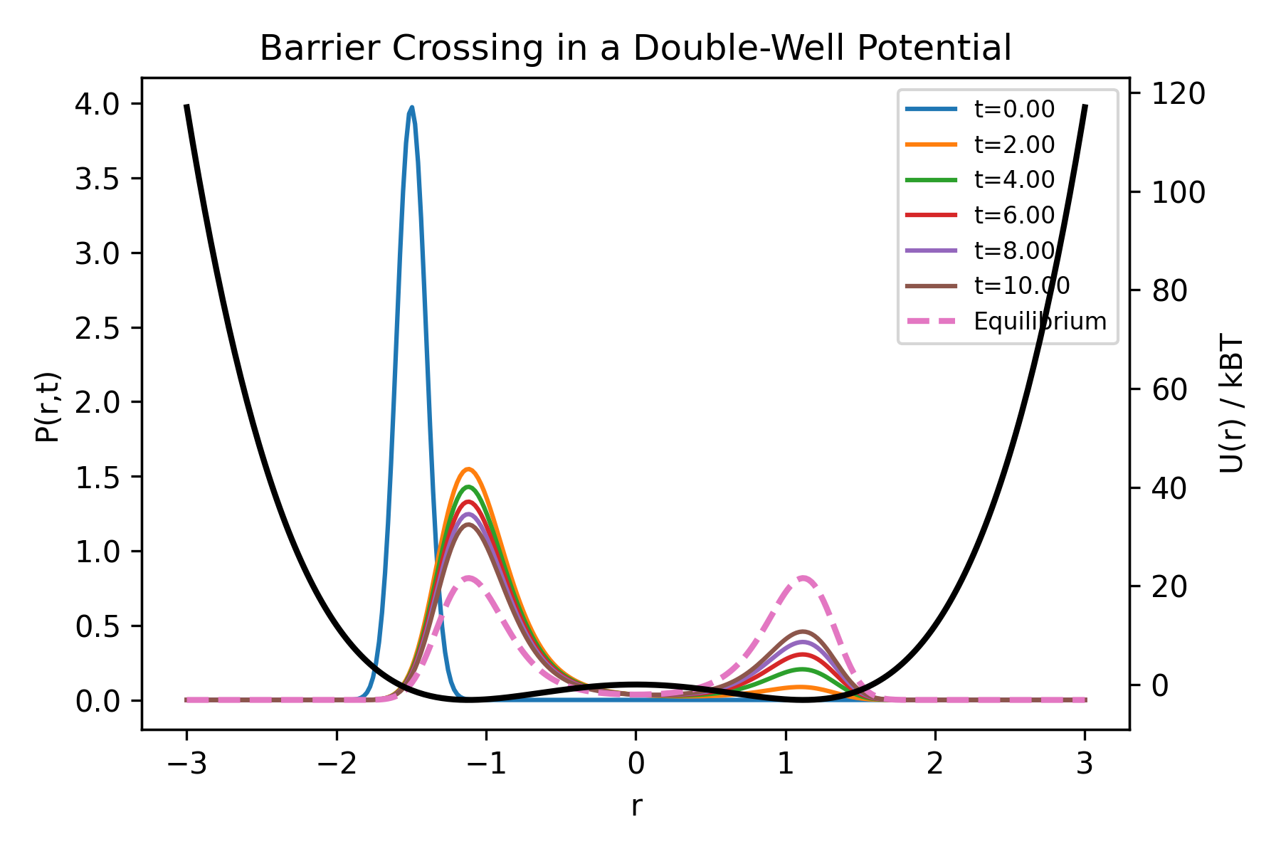
Example: Diffusion in a Double-Well Potential

A paradigmatic example illustrating the dynamics governed by the Smoluchowski equation is diffusion in a double-well potential. This system exhibits metastability and barrier-crossing dynamics, which are central in many physical, chemical, and biological processes. A simple symmetric double-well potential can be defined as:

$U(r) = a r^4 - b r^2,$
with $a > 0$ and $b > 0$ .

This potential has:

two minima at $r = \pm \sqrt{\frac{b}{2a}}$ ,
a maximum (energy barrier) at $r = 0$ .

The barrier height is given by:

$\Delta U = \frac{b^2}{4a}.$

The particle tends to localize in one of the two wells due to thermal fluctuations. Occasionally, it acquires enough thermal energy to cross the barrier and transition to the other well.

This process is governed by the competition between:

thermal energy $k_B T$ ,
barrier height $\Delta U$ .

The stationary solution of the Smoluchowski equation is:

$P_{\text{eq}}(r) \propto e^{-U(r)/(k_B T)}.$

For the double-well potential, this results in a bimodal distribution with two peaks at the minima.

The time-dependent solution can be expressed as:

$P(r,t) = \sum_n c_n \psi_n(r) e^{-\lambda_n t}.$

In a double-well system, the spectrum has a characteristic structure:

$\lambda_0 = 0$ corresponds to equilibrium,
$\lambda_1$ is very small and governs transitions between wells,
higher eigenvalues correspond to fast intra-well relaxation.

The slowest timescale,

$\tau \sim \frac{1}{\lambda_1},$ is associated with barrier crossing.

In the limit of a high barrier ( $\Delta U \gg k_B T$ ), the transition rate between wells is approximately given by Kramers’ formula:

$k \approx \frac{D}{2\pi} \sqrt{ \left| \frac{U''(r_{\text{max}})}{U''(r_{\text{min}})} \right| }, e^{-\Delta U/(k_B T)},$

where:

$r_{\text{min}}$ is the position of a minimum,
$r_{\text{max}}$ is the position of the barrier top.

This expression highlights the exponential dependence of the transition rate on the barrier height.

The code for this example is reported in the appendix.

Applications

Double-well diffusion models appear in many contexts:

chemical reactions (reactant $\leftrightarrow$ product),
protein conformational changes,
bistable systems in soft matter,
stochastic resonance and noise-driven switching.

Conclusion

The Smoluchowski equation provides a powerful framework to describe diffusion in a potential landscape. While analytical solutions exist only for simple potentials, the equation admits a spectral decomposition that reveals the relaxation dynamics of the system.

In practice, numerical methods based on conservative discretizations of the probability flux are essential for studying realistic systems.

APPENDIX

The Python program for the simulation of the barrier crossing in a double-well potential.

# ================================================================
#  Barrier Crossing in a Double-Well Potential
#  ---------------------------------------------------------------
#  Numerical solution of a 1D diffusion (Fokker–Planck) equation
#  in an external potential landscape.
#
#  The program simulates the time evolution of a probability
#  density P(r,t) under the influence of:
#      - Diffusion
#      - External potential U(r)
#
#  Physical Model
#  --------------
#  The system is described by the Fokker–Planck equation:
#
#      ∂P/∂t = ∂/∂r [ D ( ∂P/∂r + (1/kBT) P ∂U/∂r ) ]
#
#  where:
#      P(r,t)  : probability density
#      D       : diffusion coefficient
#      U(r)    : external potential (double-well)
#      kBT     : thermal energy
#
#  The potential U(r) is chosen as a symmetric double-well:
#
#      U(r) = a (r^2 - b)^2
#
#  This creates two stable minima separated by an energy barrier.
#
#  Numerical Method
#  ----------------
#  - Spatial discretization: finite differences
#  - Time integration: explicit Euler scheme
#  - Boundary conditions: absorbing (P = 0 at boundaries)
#
#  Features
#  --------
#  - Simulation of metastability and barrier crossing
#  - Visualization of probability evolution over time
#  - Comparison with equilibrium Boltzmann distribution
#  - Overlay of potential energy landscape
#  - Optional saving of figures for publication
#
#  Physical Insight
#  ----------------
#  - Fast relaxation occurs within each well
#  - Slow transitions occur across the barrier
#  - Timescale separation depends exponentially on barrier height:
#
#        τ  ~  exp(ΔU / kBT)
#
# ================================================================
#  Author: D. Roccatano
#  This code was developed with the assistance of OpenAI ChatGPT
#  (version GPT-5.3, 2026) for code generation and explanations.
#
#  Date: 2025
#  License: MIT
# ================================================================

import numpy as np
import matplotlib.pyplot as plt

# ----------------------------
# Parameters (tuned for Kramers regime)
# ----------------------------
N = 300
L = 3.0
#D = 0.2
kBT = 0.3
Tmax = 10.0
dt = 1e-4
steps = int(Tmax/dt)

a = 1.0
#b = 4.0

kBT = 0.5
b = 2.5
D = 0.5

# ----------------------------
# Grid
# ----------------------------
r = np.linspace(-L, L, N)
dr = r[1] - r[0]

# ----------------------------
# Potential
# ----------------------------
U = a*r**4 - b*r**2
dU = 4*a*r**3 - 2*b*r

# ----------------------------
# Initial condition (left well)
# ----------------------------
P = np.exp(-(r + 1.5)**2 / 0.02)
P /= np.sum(P)*dr

# ----------------------------
# Store snapshots
# ----------------------------
snapshots = []
times = []

snapshot_steps = np.linspace(0, steps-1, 6, dtype=int)

# ----------------------------
# Time evolution
# ----------------------------
for n in range(steps):

    J = np.zeros(N)

    for i in range(1, N-1):
        dU_half = 0.5*(dU[i] + dU[i+1])
        P_half = 0.5*(P[i] + P[i+1])
        dP = (P[i+1] - P[i])/dr

        J[i] = -D*(dP + (1.0/kBT)*dU_half*P_half)

    # reflecting boundaries
    J[0] = 0.0
    J[-1] = 0.0

    P_new = P.copy()
    for i in range(1, N-1):
        P_new[i] = P[i] - dt/dr*(J[i] - J[i-1])

    P_new /= np.sum(P_new)*dr
    P = P_new

    if n in snapshot_steps:
        snapshots.append(P.copy())
        times.append(n*dt)

# ----------------------------
# Plot
# ----------------------------
fig, ax1 = plt.subplots(figsize=(6,4))

for i, snap in enumerate(snapshots):
    ax1.plot(r, snap, label=f"t={times[i]:.2f}")

# equilibrium
Peq = np.exp(-U/kBT)
Peq /= np.sum(Peq)*dr
ax1.plot(r, Peq, '--', linewidth=2, label="Equilibrium")

ax1.set_xlabel("r")
ax1.set_ylabel("P(r,t)")
ax1.legend(fontsize=8)

# potential (scaled)
ax2 = ax1.twinx()
ax2.plot(r, U/kBT, 'k', linewidth=2)
ax2.set_ylabel("U(r) / kBT")

plt.title("Barrier Crossing in a Double-Well Potential")

plt.tight_layout()
plt.savefig("double_well_barrier_crossing.png", dpi=300)
plt.show()
plt.show()

M	T	W	T	F	S	S
						1
2	3	4	5	6	7	8
9	10	11	12	13	14	15
16	17	18	19	20	21	22
23	24	25	26	27	28	29
30	31

"… I seem […] only like a boy playing on the sea-shore, and diverting myself in now and then finding a smoother pebble or a prettier shell than ordinary, whilst the great ocean of truth lay all undiscovered before me". – Isaac Newton.

The Smoluchowski Diffusion Equation

Potential of Mean Force

Smoluchowski Equation

Flux Formulation

Separation of Variables

Eigenvalue Problem and Transformation

General Solution

Numerical Solution

Example: Diffusion in a Double-Well Potential

Applications

Conclusion

APPENDIX

Leave a comment Cancel reply

Potential of Mean Force

Smoluchowski Equation

Flux Formulation

Separation of Variables

Eigenvalue Problem and Transformation

General Solution

Numerical Solution

Example: Diffusion in a Double-Well Potential

Applications

Conclusion

APPENDIX

Share this:

Related

Leave a comment Cancel reply