I have recently written, for WIREs Computational Molecular Science, a review article on the use of Principal Component Analysis (PCA) in the study of dynamical systems, with a particular focus on molecular dynamics (MD) simulations of biomolecules [1]. The aim of this work is to provide a clear and practical overview of how PCA has become a central tool for extracting meaningful collective motions from high-dimensional simulation data, and how modern methodological extensions continue to expand its capabilities.
Continue readingScience Topics

RaPenduLa: Una Video piattaforma Fai-Da-Te Per Studiare Oscillazioni Meccaniche
AGGIORNAMENTO 2: Un primo articolo sulla Rapendula è stato pubblicato l’8 gennaio 2026 [1] sul The European Journal of Physics .
AGGIORNAMENTO1: Nel maggio 2025, il progetto ha ottenuto riconoscimento vincendo il 1° premio nel concorso Instructables All Things Pi. Un grande grazie al team di Instructables!
Qualche giorno fa ho pubblicato un nuovo progetto educativo sul mio sito Instructables. Il dispositivo, che ho battezzato RaPenduLa (dalle iniziali in inglese di RaspPi Pendulum Laboratory), è stato ribattezzato in italiano CAMPO (Computer Analisi Moto Pendolare Oscillante) grazie a un suggerimento di ChatGPT. Ma, come direbbe Shakespeare, ‘What’s in a name? That which we call a rose by any other name would smell as sweet’: il cuore del progetto è infatti una piattaforma video per lo studio delle oscillazioni meccaniche. Utilizzando un Raspberry Pi Zero W2 dotato di modulo fotocamera, il sistema registra ad alta velocità il movimento dei pendoli. Poi, con un’analisi video basata su Python e OpenCV, RaPenduLa è in grado di tracciare il percorso preciso della punta del pendolo, visualizzandone il comportamento oscillatorio in 2D.
Continue readingShare this:

Easter 2025: Exploring Egg-Shaped Billiards
It has become a recurrent habit for me to write a blog on the shape of eggs to wish you a Happy Easter. Not repeating oneself and finding a new interesting topic is a brainstorming exercise of lateral thinking and a systematic search in literature to find an interesting connection. This year, I wanted to explore an idea that has been lurching in my mind for some time for other reasons: billiards.
I used to play snooker from time to time with some old friends. I am a far cry from being even an amateur in the billiard games, but I had a lot of fun verifying the laws of mechanics on a green table. I soon discovered that studying the dynamics of bouncing collision of an ideal cue ball in billiards of different shapes keeps brilliant mathematicians and physicists engaged in recreational academic studies and important theoretical implications.
Continue readingShare this:

RaPenduLa: A DIY Video Platform for Exploring Mechanical Oscillations
UPDATE2: On 8 January 2026, a paper on Rapendula was published in the European Journal of Physics [1].
UPDATE 1: In May 2025, the project achieved recognition by winning first prize in the Instructables contest “All Things Pi.” A big thank you to the Instructables teams!
I have recently published another educational project on my Instructables website. I called the device RaPenduLa for the RaspPi Pendulum Laboratory, and it is a video platform for studying mechanical oscillations. It uses a Raspberry Pi Zero W2 equipped with a camera module to record the motion of pendulums at high speed. The interesting part happens through video analysis: using Python and the fantastic OpenCV library, RaPenduLa can track the precise path of a pendulum’s tip and help visualize its oscillatory behavior in two dimensions.
Continue readingShare this:

Season’s Greetings with Diffusion-Limited Aggregation!
As the year comes to a close, let us take a moment to reflect on the beauty of nature and the profound patterns that can arise from simple rules. Inspired by the Diffusion-Limited Aggregation (DLA) simulation—a concept that creates mesmerizing structures from chaotic randomness—we find parallels between its patterns and the essence of the holiday season.
The animation featured here was created using my DLA simulator, written in Awk, my favorite programming language. This program simulates the deposition of randomly diffusing particles in two dimensions. In this case, it mimics the formation of snowflakes or coriander-like clusters, with particles meandering through randomness to form intricate fractal structures.
These patterns remind us how small, individual efforts can come together to create something extraordinary. Be it family gatherings, acts of kindness, or moments of generosity, each step contributes to a larger, beautiful picture—much like how particles aggregate to form stunning natural structures such as snowflakes, coral reefs, or mineral deposits.
Wishing You:
🎄 Fractal Joy: Let your happiness grow in beautiful and unexpected ways.
🌟 Boundless Creativity: Like the Moore and von Neumann neighborhoods in the simulation, embrace different perspectives to expand your horizons.
❄️ Peace and Harmony: May your life’s matrix be filled with meaningful connections and serene moments.
May your holidays be filled with love, joy, and wonder — and may your 2024 be as inspiring as the intricate patterns of life itself!
Happy Holidays! 🌟
Share this:

How Surfactant Chain Length Shapes Protein Binding
Surfactants are everywhere in protein science — from biochemical laboratories to industrial detergents. Among them, sodium dodecyl sulfate (SDS) is perhaps the most famous (or infamous), widely used for its ability to bind, deactivate, and often denature proteins. Despite decades of experimental and theoretical work, the molecular details of how surfactants bind to protein surfaces are still not fully understood. In my recent study, “Binding Dynamics of Linear Alkyl-sulfates of Different Chain Lengths on a Protein Surface” [1], I have explored this problem using molecular dynamics (MD) simulations, focusing on how the length of the surfactant’s hydrocarbon chain influences protein binding.
Continue readingShare this:

Chlorophyll in Tight Spaces: How Silica Nanoconfinement Stabilizes Photosynthetic Pigments
In a recent molecular dynamics study [1] in collaboration with Prof. K. J. Karki (Department of Physics, Guangdong Technion-Israel Institute of Technology in China), we explored how EthylChlorophyllide a behaves when confined between two silica surfaces — a situation relevant for artificial photosynthesis, nanomaterials, and bio-inspired light-harvesting systems. Chlorophylls are among the most important molecules on Earth. They enable plants, algae, and photosynthetic bacteria to convert sunlight into chemical energy. Yet, outside their natural protein environment, chlorophyll molecules are fragile as they can easily lose their central magnesium ion (demetallation), they degrade under light, and they tend to aggregate uncontrollably in solution.
In natural photosynthetic systems, proteins protect and organize chlorophylls. Reproducing this level of control in artificial systems remains a major challenge. One promising strategy is nanoconfinement — trapping chlorophyll derivatives inside well-defined inorganic structures such as silica nanopores.
Continue readingShare this:

Look at the Rainbow in a Soap Film: A simple STEM Project
My heart leaps up when I behold
A rainbow in the sky:
So was it when my life began;
So is it now I am a man;
So be it when I shall grow old,
Or let me die!
The Child is father of the Man;
And I could wish my days to be
Bound each to each by natural piety.William Wordsworth, March 26, 1802
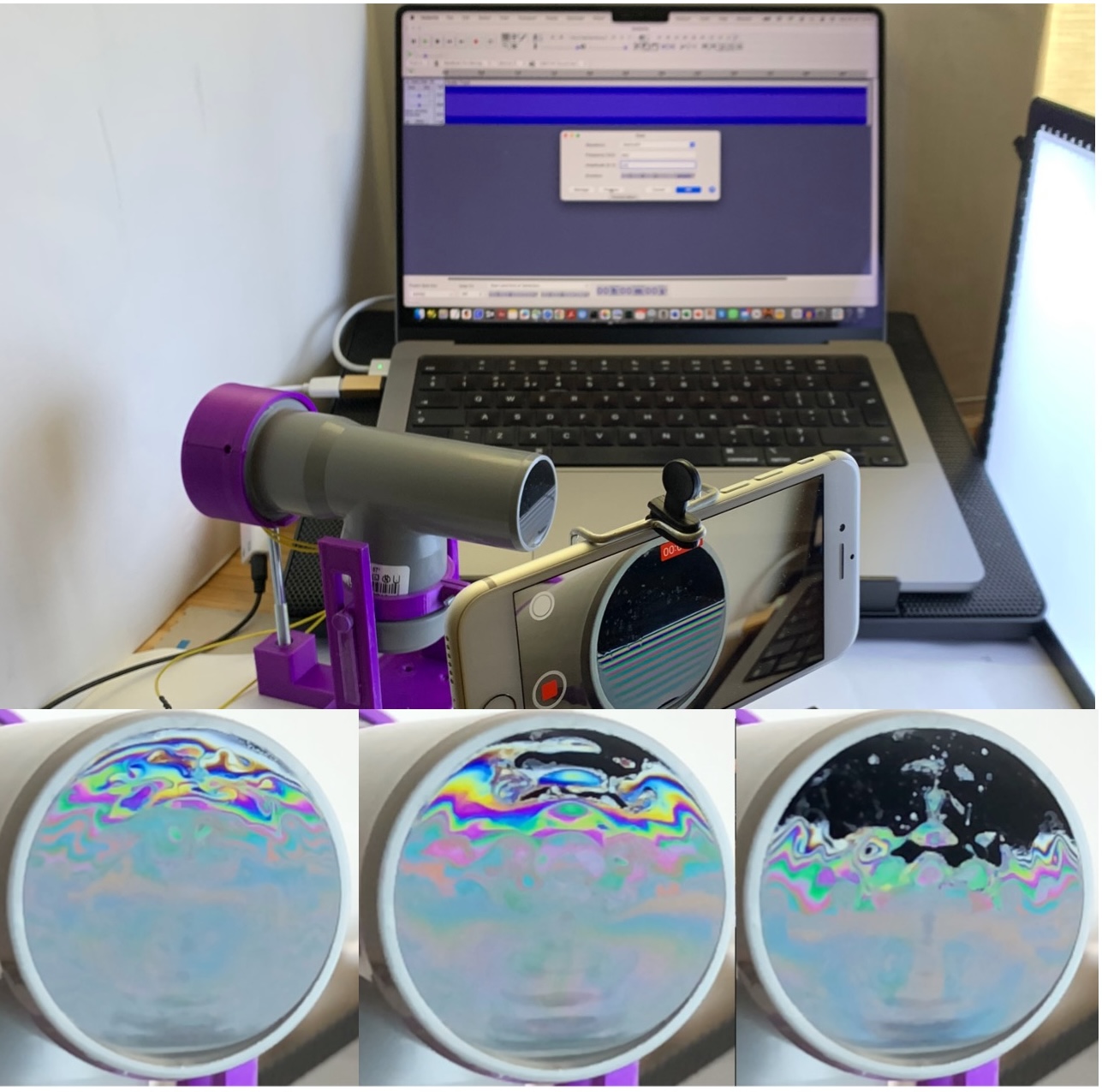
I couldn’t resist citing the beautiful poetry by Wordsworth about the rainbow to introduce my new Instructable, ‘Explore the Physics of Soap Films with the SoapFilmScope.’ I got the idea for this project by reading an article by Gaulon et al. [1]. The authors describe in detail the use of soap film as an educational aid to explore interesting effects in the fluid dynamics of this system. In particular, they examine the impact of acoustic waves on the unique optical properties of the film. In this Instructable, we have designed a device called the SoapFilmScope to perform these experiments. This tutorial will guide you through the process of creating this device, showcasing the mesmerizing interaction between sound waves and liquid membranes. The SoapFilmScope offers an engaging way to explore the physics of acoustics, light interference, and fluid dynamics.
When a sound wave travels through the tube and vibrates the soap film, it creates dynamic patterns through several fascinating mechanisms:
The device consists of a vertical soap film delicately suspended at the end of a tube obtained from a PVC T-shaped fitting that you can get from any DIY store. By attaching a small inexpensive speaker to it, you can let the film dance to the rhythm of the music.
Share this:

Retro Programming Nostalgia VI: Exploring the Hyperspace
Henk Rogers: Um, I like Pascal. Assembler is my go-to. But never underestimate…
Alexey Pajitnov: …the power of BASIC.
From the movie Tetris (2023).
It has been a long while that I wanted to write this article. The usual motivation is to propose another of my BASIC programming explorations performed in the 80s on my Philips MSX VG-8010 and Amiga 500 microcomputer. The exploration was encouraged by the reading of another of the brilliant articles by A. K. Dewdney in his column “Ricreazioni al Calcolatore” (Computer Recreation) of Le Scienze, the edition in Italian of Scientific American [1]. Dewdney’s article was inspired by the beautiful book by Thomas F. Banchoff [2] who pioneered in the early 1990s the study using computer graphics of hyperdimensional objects.
Continue readingShare this:

Exploring Disordered Proteins: A Study on Flexible Peptides
Proteins are not always rigid structures. Many of their most important parts — linkers, loops, and disordered regions — are highly flexible, constantly changing shape in solution. To understand how these regions behave, scientists often study short model peptides that capture the essential physics of flexibility. In a new article [1], I have explored the behavior of glycine- and serine-rich octapeptides using molecular dynamics simulations combined with concepts from FRET (Förster Resonance Energy Transfer) spectroscopy (see also my previous post).
Continue reading
