Ettore Majorana e L’Equazione di Fermi-Thomas

Perché al mondo vi sono varie categorie di scienziati, gente di secondo e terzo rango, che fa del suo meglio ma non va lontano; c’è anche gente di primo rango, che arriva a scoperte di grande importanza, fondamentali per lo sviluppo della scienza. Ma poi ci sono i geni, come Galileo e Newton. Ebbene Ettore era uno di quelli. (Commento di Enrico Fermi alla notizia della scomparsa di Majorana)

Qualche tempo fa ho rivisto il film su Raiplay in due parti diretto da Gianni Amelio, I ragazzi di via Panisperna. Si tratta di un’opera trasmessa dalla Rai alla fine degli anni Ottanta, molto bella e ben realizzata, che racconta le vicende che portarono alla formazione, negli anni Venti e Trenta, del celebre gruppo di Enrico Fermi presso l’Istituto di Fisica di via Panisperna, all’Università di Roma. Il film si concentra in particolare sulle figure di Ettore Majorana (interpretato da Andrea Prodan) e di Enrico Fermi (Ennio Fantastichini).

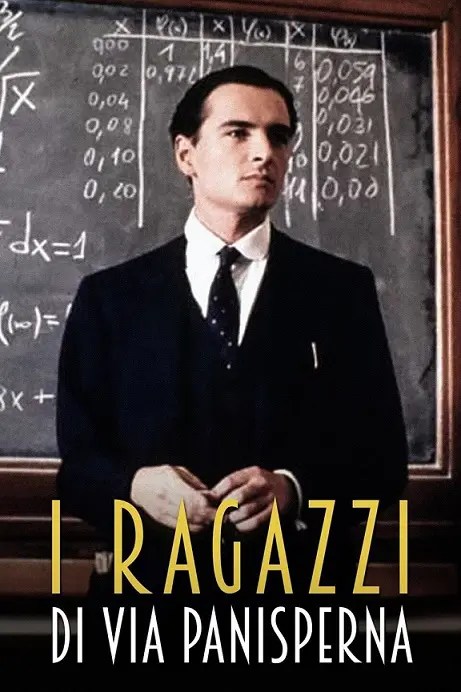
L’incontro tra i due è raccontato attraverso una scena memorabile, in cui Majorana è mostrato alla lavagna mentre lavora alla soluzione di un’equazione differenziale (quella che diventerà nota come equazione di Thomas-Fermi), assegnata da Fermi come prova d’ammissione al suo gruppo. Majorana viene osservato nell’aula dallo stesso Fermi, che, fingendosi uno studente del gruppo, gli rivela di essere alle prese con quella stessa equazione da una settimana, insieme ad altri due colleghi. Nella scena successiva, Amelio mette magistralmente in luce la brillantezza di Majorana, che svela a Fermi di aver risolto il problema in una sola notte. La recente raccolta e pubblicazione dei suoi scritti inediti (i Quadernetti, una serie di appunti curati risalenti al periodo dei suoi studi di fisica) a cura del Prof. Salvatore Esposito (Università di Napoli) ha rivelato ulteriori dettagli su questo episodio. Si tratta, in effetti, di una vera e propria competizione matematica tra due geni, nella quale Majorana dimostrò una superiorità più volte riconosciuta dallo stesso Fermi.

La visione del film mi ha spinto ad approfondire lo studio della soluzione numerica di questa equazione. In questo articolo, vorrei condividere alcune riflessioni su questa equazione e sul problema che Fermi ha posto alla brillante Majorana.

Continue reading

Easter 2026: The Patterns on Coturnix Egg

Last year, after a series of unsuccessful attempts and acquiring three incubators across two countries, my youngest son’s unwavering determination finally paid off.  From a batch of twelve mixed quail eggs, seven hatched successfully, marking the start of our new venture into farm animal husbandry.  Currently, we’ve settled for manageable pets like a Siberian hamster, an aquarium, and pond fish, plus several rounds of stick insects, mantises, and spiders, along with their grasshopper and locust food supplies.  However, quail care is more demanding. While our sons’ happiness is undoubtedly the most important reward, the delicious eggs produced by our farm breeding activity are equally rewarding for the whole family.  It’s particularly satisfying collecting every evening the two expected eggs from the punctual quail hens and admiring their different sizes and pigmentation like beautiful little gems.

If you’re still reading, you’ve probably guessed the main topics of my traditional Easter blog: quail eggs and their shapes and patterns.

Continue reading

The Numerical Solution of Differential Equation using the Shooting Method

Boundary value problems (BVPs) for ordinary differential equations arise naturally in many areas of physics, engineering, and applied mathematics. Classical examples include the vibration of strings, heat conduction in solids, and quantum mechanical bound states. Unlike initial value problems (IVPs), where all conditions are specified at a single point, BVPs impose constraints at different points of the domain, making them significantly more challenging to solve both analytically and numerically.

The shooting method is one of the most intuitive and historically rooted techniques for tackling such problems. Its central idea is simple: transform a boundary value problem into an initial value problem by guessing the missing initial conditions, then iteratively refine this guess until the solution satisfies the boundary conditions at the other end. The method is often illustrated through a ballistic analogy—one “shoots” from the initial point and adjusts the trajectory until the target is hit. Although the shooting method was formalized only in the 20th century, its conceptual foundations can be traced back much earlier. The study of differential equations in the 18th and 19th centuries by mathematicians such as Leonhard Eulerand Joseph-Louis Lagrange already revealed the difficulty of boundary value problems in mechanics and astronomy. At that time, analytical solutions were often unavailable, and practitioners relied on approximation strategies that implicitly resembled “trial-and-error” approaches. A decisive step toward the modern shooting method came with the development of reliable numerical solvers for initial value problems around 1900, notably through the work of Carl Runge and Martin Kutta. Their methods provided the computational backbone needed to integrate differential equations accurately from a given starting point. This made it feasible to implement the idea of repeatedly “shooting” with different initial guesses. The method gained wider recognition and systematic treatment in the mid-20th century, alongside the emergence of numerical analysis as a distinct discipline. Influential mathematicians such as Richard Courant contributed to the theoretical understanding of boundary value problems, while the increasing availability of digital computers transformed the shooting method into a practical and widely used computational tool.

Today, the shooting method remains a cornerstone in the teaching of numerical methods due to its conceptual clarity and direct connection to physical intuition. While more robust techniques—such as finite difference and finite element methods—are often preferred for complex or stiff problems, the shooting method continues to play an important role in applications ranging from classical mechanics to quantum physics, where it is frequently used to determine eigenvalues and admissible solutions.

In this blog, I will give an example of the application of the method to the solution of the Thomas-Fermi and Thomas-Fermi-Dirac equations.

Continue reading

The Smoluchowski Diffusion Equation

The Smoluchowski diffusion equation describes the time evolution of the probability density function (PDF) of a particle undergoing overdamped Brownian motion in a potential energy landscape. It is a central equation in statistical mechanics, soft matter physics, and chemical physics.

Its origins trace back to the early 20th century, in the context of the theoretical understanding of Brownian motion. Following the seminal work of Albert Einstein in 1905, who provided a statistical description of diffusion and established a quantitative link between microscopic fluctuations and macroscopic transport, further developments aimed to incorporate external forces and interactions. In 1916, Marian Smoluchowski extended Einstein’s framework by considering particles subjected to systematic forces arising from a potential field. His formulation led to what is now known as the Smoluchowski equation, effectively describing diffusion in the overdamped (high-friction) limit where inertial effects can be neglected. This marked a crucial step toward connecting stochastic motion with deterministic drift. A complementary perspective emerged through the work of Paul Langevin (1908), who introduced a stochastic differential equation for particle motion, explicitly incorporating random forces. The equivalence between the Langevin description and the corresponding evolution equation for probability densities—later formalized as the Fokker–Planck equation—provided a deep and unifying framework. The general mathematical structure of such evolution equations was further clarified by Adriaan Fokker and Max Planck in the early 20th century, leading to the modern formulation of the Fokker–Planck equation. The Smoluchowski equation can be viewed as a specific limit of this more general framework. Later, in the 1940s, Hendrik Anthony Kramers applied these ideas to chemical reaction rates, analyzing barrier crossing in potential landscapes. His work revealed how transition rates depend exponentially on the energy barrier height, establishing the foundation of what is now known as Kramers’ theory—an essential concept for understanding metastability and rare events.

In this article, we consider the one-dimensional (1D) case, where a particle moves along a coordinate r under the influence of a potential of mean force U(r).

Continue reading

Understanding the Discrete Fourier Transform in Signal Analysis

In previous posts on this blog I have already introduced the Fourier series and the Fourier transform, following their historical development from Joseph Fourier’s original work on heat conduction to their modern role in physics, engineering, and signal analysis. Rather than repeating that material here, I will take it as a starting point.

When we look at a signal — a sound wave, a vibration, or even a curve drawn by hand — we usually perceive it as a function of time or space. However, very often the most relevant information is not immediately visible in this representation. It is hidden in the frequencies that compose the signal, and in how strongly each of them contributes.

This is precisely the idea behind the Discrete Fourier Transform (DFT): to decompose a discrete signal into a finite sum of harmonic components, each characterized by an amplitude and a phase. Conceptually, the DFT is not a new theory, but a practical bridge between the continuous Fourier framework and the realities of digital data, measurements, and numerical simulations.

Rather than starting from abstract formulas, in this post I adopt a visual and experimental approach. The discussion is supported by an interactive program that allows one to draw an arbitrary signal and explore its harmonic content, and by a practical electronics project where Fourier analysis is applied to real sound and noise signals.

Continue reading

Retro Programming Nostalgia VIII: 1926-2026 l’equazione di Schrödinger e la struttura elettronica dell’atomo d’idrogeno

Quest’anno ricorre l’anniversario della pubblicazione dell’articolo di Edwin Schrödinger (1887-1961) in cui viene introdotta la sua famosa equazione. Prendendo spunto da questa occasione, ho ripescato e rinnovato uno dei miei antichi progetti di programmazione in BASIC con i miei microcomputer negli anni ’80. Di nuovo il microcomputer era il mio amato Phillips MSX, di cui ho parlato in altri blog. Studiando chimica, non potevo non essere attratto dalla bellezza e dall’eleganza delle soluzioni dell’equazione di Schrödinger per l’atomo d’idrogeno. Inspirato dal libro (S. Marseglia, La Chimica col personal computer pubblicato dalla Muzzio) in cui mostrava alcuni esempi di programmi in BASIC per la chimica, decisi di imbarcarmi nell’impresa e usare l’MSX e poi l’Amiga Basic Basic per provare a riprodurre le bellissime visualizzazioni degli orbitali molecolari che vedevo nei libri di chimica universitari. Ma prima di questo vediamo di tornare a contenuto dell’articolo di Schrödinger.

Continue reading

Christmas 2025: Growing Christmas Trees from Factorials

Christmas is a time for traditions, decorations, and—at least for some of us—quiet moments spent playing with ideas. In that spirit, this post is a small seasonal diversion: a recreational exploration of large factorial numbers, their historical computation, and an unusual way to see them. The inspiration comes from an old but delightful article by the great recreational mathematician  Martin Gardner, titled “In which a computer prints out mammoth polygonal factorials” (Scientific American, August 1967), in which he discusses the astonishing growth of the function

n! = 1 \cdot 2 \cdot 3 \cdots n

and the surprising difficulty computers once faced when trying to compute it for even modest values of n.

In this post, I will briefly describe the Smith bin algorithm for computing large factorials and present the result for the number 2025, arranged in a geometric form. After all, if numbers are going to grow explosively, why not let them grow into Christmas trees for 2025?

Continue reading

Principal Component Analysis: Key to Analyzing Biomolecular Dynamics

I have recently written, for WIREs Computational Molecular Science, a review article on the use of Principal Component Analysis (PCA) in the study of dynamical systems, with a particular focus on molecular dynamics (MD) simulations of biomolecules [1]. The aim of this work is to provide a clear and practical overview of how PCA has become a central tool for extracting meaningful collective motions from high-dimensional simulation data, and how modern methodological extensions continue to expand its capabilities.

Continue reading

RaPenduLa: Una Video piattaforma Fai-Da-Te Per Studiare Oscillazioni Meccaniche

Qualche giorno fa ho pubblicato un nuovo progetto educativo sul mio sito Instructables. Il dispositivo, che ho battezzato RaPenduLa (dalle iniziali in inglese di RaspPi Pendulum Laboratory), è stato ribattezzato in italiano CAMPO (Computer Analisi Moto Pendolare Oscillante) grazie a un suggerimento di ChatGPT. Ma, come direbbe Shakespeare, ‘What’s in a name? That which we call a rose by any other name would smell as sweet’: il cuore del progetto è infatti una piattaforma video per lo studio delle oscillazioni meccaniche. Utilizzando un Raspberry Pi Zero W2 dotato di modulo fotocamera, il sistema registra ad alta velocità il movimento dei pendoli. Poi, con un’analisi video basata su Python e OpenCV, RaPenduLa è in grado di tracciare il percorso preciso della punta del pendolo, visualizzandone il comportamento oscillatorio in 2D.

Continue reading

Easter 2025: Exploring Egg-Shaped Billiards

It has become a recurrent habit for me to write a blog on the shape of eggs to wish you a Happy Easter. Not repeating oneself and finding a new interesting topic is a brainstorming exercise of lateral thinking and a systematic search in literature to find an interesting connection. This year, I wanted to explore an idea that has been lurching in my mind for some time for other reasons: billiards.

I used to play snooker from time to time with some old friends. I am a far cry from being even an amateur in the billiard games, but I had a lot of fun verifying the laws of mechanics on a green table. I soon discovered that studying the dynamics of bouncing collision of an ideal cue ball in billiards of different shapes keeps brilliant mathematicians and physicists engaged in recreational academic studies and important theoretical implications.

Continue reading