In 1926, the Austrian physicist Erwin Schrödinger (1887-1961) made a fundamental mathematical discovery that had a profound impact on the study of the molecular world (in 1933, Schrödinger was awarded the Nobel Prize in Physics just seven years later, his breakthrough discovery). He discovered that a quantum system’s state composed of particles (such as electrons and nucleons) could be described by postulating the existence of a function of the particle coordinates and time, called state function or wave function (
Nowadays, computational quantum chemistry has surged to a level of a fundamental research discipline in chemistry and material science. In recognition of their contribution to the advancement of science, the pioneers of this discipline, Prof. Walter Kohn and Prof. John A. Pople, have been awarded the 2008 Nobel Prize in chemistry.
In this primer, we will study analytical and numerical solutions of SE for simple quantum systems in stationary conditions, e.g. whose state does not change with time. For this purpose, we will use the time-independent form of SE. This condition is an excellent approximation to describe the state of molecular systems.
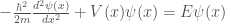
The time-independent SE is given in its compact form by the equation.

where the 


We now look more in detail at the Hamiltonian operator. For the sake of simplicity, we will limit ourselves to consider only a mono-dimensional physical system, namely a system defined only along a reference x-axis. Therefore, the wave function depends only on by x or 


This differential equation can be solved analytically for different types of potentials. A simple classical example is a particle in a one-dimension box within infinitely repulsive barriers.
In this case, the value of 


Derivation of the wavefunction
The one-dimension SE is a linear second-order differential equation with solutions

using the Euler relation

we can write

or called 


by substituting in SE with

we obtain

that gives

the quantised total energy of the system.
Now we estimate the values of constant k, C, and D of the solution.
By applying the boundary conditions

we obtain for x=0 that

It is more convenient to represent the parameter k as a circular frequency with 

For x=L the solution gives

This is accomplished for 

and

We still need to calculate the value of the constant C. As the square of the wave function 

Using this integral we can find the value of C that normalize the function. The integral 

as 


so we have that
taking the last integral in the second member of the equation to the first member we have

but the first term in the second member is equal to zero and the second equal to L, hence

Therefore from Equ. (1), we have

and 
Therefore the wavefunctions of a particle in a box are given by

and the associated energies are

The quantum number n is an integer associated with the different energy levels of the particle. Larger n values correspond to higher energy levels of the system. Also, note in the graphs the increase in the number of nodes in the wave function with the increase of the value of n.
In Figure 2, the wavefunctions for the first three energy level of the particle in a box are shown.

The separation between the adjacent energy level with quantum number $n$ and $n+1$ is

The probability density for a particle in a box is given by the square of the wavefunction as follows

and the probability to find the particle in a region ![[x_1,x_2]](https://s0.wp.com/latex.php?latex=%5Bx_1%2Cx_2%5D&bg=ffffff&fg=444444&s=0&c=20201002)

READINGS
- Atkins, P. and Paula, J. (2010) Physical Chemistry. 9th Edition, W. H. Freeman Co., New York.
- I. Levine. Quantum Chemistry. VI edition. Pearson International edition.


Esercizio interessante (problemi unidimensionali in meccanica quantistica nonrelativistica). Tempo addietro ne avevo svolto uno simile. Precisamente, un oscillatore armonico unidimensionale, però considerando uno stato quantistico descritto da una funzione d’onda che pur essendo normalizzabile, non si annulla all’infinito: http://www.extrabyte.info/2019/03/01/gli-stati-ghost-delloscillatore-armonico-unidimensionale/
Una tale soluzione ha un significato fisico? A me sembra di no, per la semplice ragione che si dovrebbe congetturare l’esistenza di un processo di tunnelling in presenza di un potenziale divergente all’infinito.
LikeLike
Grazie Marcello per il tuo commento. I tuoi posts sono molto interessanti e decisamente piu’ avanzati del mio. Aggiungero’ dei link per chi e’ interessato ad approfondire l’argomento. Lo scopo di questi miei articoli e’ quello di dare una introduzione a concetti di base della chimica fisica e, anche, una occasione per presentare qualche vecchio programma in BASIC sviluppato in passato per scopi didattici.
Riguardo la tua domanda, in realta soluzioni semplici come questa della equazioni di SE non dipendente dal tempo sono state molto importanti nello sviluppo della chimica teorica prima dell’avvento dei calcolatori elettronici. In una seconda parte del mio articolo (e grazie al tuo commento mi hai dato lo stimolo per scriverlo!) mostrerò un esempio classico di applicazione con il solito programmino aggiunto per fare qualche esperimento computazionale.
LikeLike
Ciao Danilo.
Im paio si precisazioni e errata corrige:
nella frase: “This function are solution of a wave equation: the so-called the Schrödinger equation (SE)”
occorre sostituire “this function” con la forma plurale “these functions”.
nella frase: “The application of the operator produce as results the same wave function multiplied for a number $E.$ This number represented the total energy state of the system (or \em eigenstate\em). This equation is also called eigenvalue equation, and, in this case, \Psi(x,y,z) is also said to be an eigenfunction of \bf \hat H with the associated \em eigenvalue,\em E. ”
ci sono alcuni tag html che non vengono correttamente letti dal browser web – vedi i segni di dollaro e \em, \b \Psi(x,y,z)
nella frase: “In this case, the value of V(x) is equal zero for and infinite in the walls.”
manca una parte della descrizione della funzione potenziale: V(x) = 0 per 0 <= x <= L
le formule :
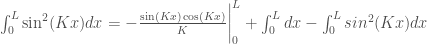
\int_{0}^L \sin^2 (x) dx = -\frac{\sin (Kx) \cos(Kx)}{K} \bigg|_{0}^L + K\int_0^L \cos^2(x) dx = -\frac{\sin (Kx) \cos(Kx)}{K} \bigg|_{0}^L + \int_0^L (1-\sin^2(Kx)) dx
e
\int_0^L \sin^2 (Kx) dx = \frac{L}{2}.
non vengono visualizzate. Compare in entrambi i casi un orribile riquadro giallo con la scritta in rosso "Formula does not parse".
Quando esegui la differenziazione della funzione d'onda in forma trigonometrica:
-\frac{\hbar^2}{2m}\left( -C\sin(kx)-D\cos(kx)\right) = E_k\left(C\sin(kx)+D\cos(kx)\right)
hai dimenticato a moltiplicare per k al quadrato il primo membro.
Spero che le mie indicazioni aiutino a migliorare la qualità della tua pagina.
grazie.
LikeLike
Ciao Alessandro, grazie infinite per i tuoi commenti. Non solo contribuiscono a migliorare la qualità della pagina, ma mi incoraggiano anche a pubblicarne di nuove!
LikeLike
Pingback: Examples of the Particle in a Box model applications |